15 Support Vector Machines
This page is a work in progress and minor changes will be made over time.
Support vector machines are a popular class of models in regression and classification settings due to their ability to make accurate predictions for complex high-dimensional, non-linear data. Survival support vector machines (SSVMs) predict continuous responses that can be used as ranking predictions with some formulations that provide survival time interpretations. This chapter starts with SVMs in the regression setting before moving to adaptions for survival analysis.
15.1 SVMs for Regression
In simple linear regression, the aim is to estimate the line \(y = \alpha + x\beta_1\) by estimating the \(\alpha,\beta_1\) coefficients. As the number of coefficients increases, the goal is to instead estimate the hyperplane, which divides the higher-dimensional space into two separate parts. To visualize a hyperplane, imagine looking at a room from a birds eye view that has a dividing wall cutting the room into two halves (Figure 15.1). In this view, the room appears to have two dimensions (x=left-right, y=top-bottom) and the divider is a simple line of the form \(y = \alpha + x\beta_1\). In reality, this room is actually three dimensional and has a third dimension (z=up-down) and the divider is therefore a hyperplane of the form \(y = \alpha + x\beta_1 + z\beta_2\).

Continuing the linear regression example, consider a simple model where the objective is to find the \(\boldsymbol{\beta} = ({\beta}_1 \ {\beta}_2 \cdots {\beta}_{p})^\intercal\) coefficients that minimize \(\sum^n_{i=1} (g(\mathbf{x}_i) - y_i)^2\) where \(g(\mathbf{x}_i) = \alpha + \mathbf{x}_i^\intercal\boldsymbol{\beta}\) and \((\mathbf{X}, \mathbf{y})\) is training data such that \(\mathbf{X}\in \mathbb{R}^{n \times p}\) and \(\mathbf{y}\in \mathbb{R}^n\). In a higher-dimensional space, a penalty term can be added for variable selection to reduce model complexity, commonly of the form
\[ \frac{1}{2} \sum^n_{i=1} (g(\mathbf{x}_i) - y_i)^2 + \frac{\lambda}{2} \|\boldsymbol{\beta}\|^2 \]
for some penalty term \(\lambda \in \mathbb{R}\). Minimizing this error function effectively minimizes the average difference between all predictions and true outcomes, resulting in a hyperplane that represents the best linear relationship between coefficients and outcomes.
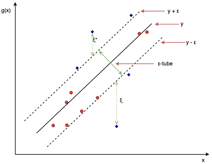
Similarly to linear regression, support vector machines (SVMs) (Cortes and Vapnik 1995) also fit a hyperplane, \(g\), on given training data, \(\mathbf{X}\). However, in SVMs, the goal is to fit a flexible (non-linear) hyperplane that minimizes the difference between predictions and the truth for individual observations. A core feature of SVMs is that one does not try to fit a hyperplane that makes perfect predictions as this would overfit the training data and is unlikely to perform well on unseen data. Instead, SVMs use a regularized error function, which allows incorrect predictions (errors) for some observations, with the magnitude of error controlled by an \(\epsilon>0\) parameter as well as slack parameters, \(\boldsymbol{\xi'} = ({\xi'}_1 \ {\xi'}_2 \cdots {\xi'}_{n})^\intercal\) and \(\boldsymbol{\xi^*} = ({\xi^*}_1 \ {\xi^*}_2 \cdots {\xi^*}_{n})^\intercal\) :
\[ \begin{aligned} & \min_{\boldsymbol{\beta},\alpha, \boldsymbol{\xi}', \boldsymbol{\xi}^*} \frac{1}{2} \|\boldsymbol{\beta}\|^2 + C \sum^n_{i=1}(\xi'_i + \xi_i^*) \\ & \textrm{subject to} \begin{dcases} g(\mathbf{x}_i) & \geq y_i -\epsilon - \xi'_i \\ g(\mathbf{x}_i) & \leq y_i + \epsilon + \xi_i^* \\ \xi'_i, \xi_i^* & \geq 0 \\ \end{dcases} \end{aligned} \tag{15.1}\]
\(\forall i\in 1,...,n\) where \(g(\mathbf{x}_i) = \alpha + \mathbf{x}_i^\intercal\boldsymbol{\beta}\) for model weights \(\boldsymbol{\beta}\in \mathbb{R}^p\) and \(\alpha \in \mathbb{R}\) and the same training data \((\mathbf{X}, \mathbf{y})\) as above.
Figure 15.2 visualizes a support vector regression model in two dimensions. The red circles are values within the \(\epsilon\)-tube and are thus considered to have a negligible error. In fact, the red circles do not affect the fitting of the optimal line \(g\) and even if they moved around, as long as they remain within the tube, the shape of \(g\) would not change. In contrast the blue diamonds have an unacceptable margin of error – as an example the top blue diamond will have \(\xi'_i = 0\) but \(\xi_i^* > 0\), thus influencing the estimation of \(g\). Points on or outside the epsilon tube are referred to as support vectors as they affect the construction of the hyperplane. The \(C \in \mathbb{R}_{>0}\) hyperparameter controls the slack parameters and thus as \(C\) increases, the number of errors (and subsequently support vectors) is allowed to increase resulting in low variance but higher bias, in contrast a lower \(C\) is more likely to introduce overfitting with low bias but high variance (Hastie, Tibshirani, and Friedman 2001). \(C\) should be tuned to control this trade-off.
The other core feature of SVMs is exploiting the kernel trick, which uses functions known as kernels to allow the model to learn a non-linear hyperplane whilst keeping the computations limited to lower-dimensional settings. Once the model coefficients have been estimated using the optimization above, predictions for a new observation \(\mathbf{x}^*\) can be made using a function of the form
\[ \hat{g}(\mathbf{x}^*) = \sum^n_{i=1} \mu_iK(\mathbf{x}^*,\mathbf{x}_i) + \alpha \tag{15.2}\]
Details (including estimation) of the \(\mu_i\) Lagrange multipliers are beyond the scope of this book, references are given at the end of this chapter for the interested reader. \(K\) is a kernel function, with common functions including the linear kernel, \(K(x^*,x_i) = \sum^p_{j=1} x_{ij}x^*_j\), radial kernel, \(K(x^*,x_i) = \exp(-\omega\sum^p_{j=1} (x_{ij} - x^*_j)^2)\) for some \(\omega \in \mathbb{R}_{>0}\), and polynomial kernel, \(K(x^*,x_i) = (1 + \sum^p_{j=1} x_{ij}x^*_j)^d\) for some \(d \in \mathbb{N}_{> 0}\).
The choice of kernel and its parameters, the regularization parameter \(C\), and the acceptable error \(\epsilon\), are all tunable hyper-parameters, which makes the support vector machine a highly adaptable and often well-performing machine learning method. The parameters \(C\) and \(\epsilon\) often have no clear apriori meaning (especially true in the survival setting predicting abstract rankings) and thus require tuning over a great range of values; no tuning usually results in a poor model fit (Probst, Boulesteix, and Bischl 2019).
15.2 SVMs for Survival Analysis
Extending SVMs to the survival domain (SSVMs) is a case of: i) identifying the quantity to predict; and ii) updating the optimization problem (Equation 15.1) and prediction function (Equation 15.2) to accommodate for censoring. In the first case, SSVMs can be used to either make survival time or ranking predictions, which are discussed in turn. The notation above is reused below for SSVMs, with additional notation introduced when required and now using the survival training data \((\mathbf{X}, \mathbf{t}, \boldsymbol{\delta})\).
15.2.1 Survival time SSVMs
To begin, consider the objective for support vector regression with the \(y\) variable replaced with the usual survival time outcome \(t\), for all \(i\in 1,...,n\):
\[ \begin{aligned} & \min_{\boldsymbol{\beta}, \alpha, \boldsymbol{\xi}', \boldsymbol{\xi}^*} \frac{1}{2} \|\boldsymbol{\beta}\|^2 + C \sum^n_{i=1}(\xi'_i + \xi_i^*) \\ & \textrm{subject to} \begin{dcases} g(\mathbf{x}_i) & \geq t_i -\epsilon - \xi'_i \\ g(\mathbf{x}_i) & \leq t_i + \epsilon + \xi_i^* \\ \xi'_i, \xi_i^* & \geq 0 \\ \end{dcases} \end{aligned} \tag{15.3}\]
In survival analysis, this translates to fitting a hyperplane in order to predict the true survival time. However, as with all adaptations from regression to survival analysis, there needs to be a method for incorporating censoring.
Recall the \((t_l, t_u)\) notation to describe censoring as introduced in Chapter 4 such that the outcome occurs within the range \((t_l, t_u)\). Let \(\tau \in \mathbb{R}_{>0}\) be some known time-point, then an observation is:
- left-censored if the survival time is less than \(\tau\): \((t_l, t_u) = (-\infty, \tau)\);
- right-censored if the true survival time is greater than \(\tau\): \((t_l, t_u) = (\tau, \infty)\); or
- uncensored if the true survival time is known to be \(\tau\): \((t_l, t_u) = (\tau, \tau)\).
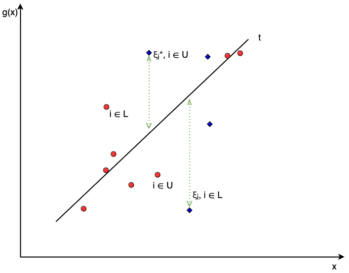
Define \(\mathcal{L}= \{i: t_i > -\infty\}\) as the set of observations with a finite lower-bounded time, which can be seen above to be those that are right-censored or uncensored. Define \(\mathcal{U}= \{i: t_i < \infty\}\) as the analogous set of observations with a finite upper-bounded time, which are those that are left-censored or uncensored.
Consider these definitions in the context of the constraints in Equation 15.3. The first constraint ensures the hyperplane is greater than some lower-bound created by subtracting the slack parameter from the true outcome – given the set definitions above this constraint only has meaning for observations with a finite lower-bound, \(i \in \mathcal{L}\), otherwise the constraint would include \(g(\mathbf{x}_i) \geq -\infty\), which is clearly not useful. Similarly the second constraint ensures the hyperplane is less than some upper-bound, which again can only be meaningful for observations \(i \in \mathcal{U}\). Restricting the constraints in this way leads to the optimization problem (Shivaswamy, Chu, and Jansche 2007) below and visualised in Figure 15.3:
\[ \begin{aligned} & \min_{\boldsymbol{\beta}, \alpha, \boldsymbol{\xi}', \boldsymbol{\xi}^*} \frac{1}{2}\|\boldsymbol{\beta}\|^2 + C\Big(\sum_{i \in \mathcal{U}} \xi_i + \sum_{i \in \mathcal{L}} \xi_i^*\Big) \\ & \textrm{subject to} \begin{dcases} g(\mathbf{x}_i) & \geq t_i -\xi'_i, i \in \mathcal{L}\\ g(\mathbf{x}_i) & \leq t_i + \xi^*_i, i \in \mathcal{U}\\ \xi'_i \geq 0, \forall i\in \mathcal{L}; \xi^*_i \geq 0, \forall i \in \mathcal{U} \end{dcases} \end{aligned} \]
If no observations are censored then the optimization becomes the regression optimization in (Equation 15.1). Note that in SSVMs, the \(\epsilon\) parameters are typically removed to better accommodate censoring and to help prevent the same penalization of over- and under-predictions. In contrast to this formulation, one could introduce more \(\epsilon\) and \(C\) parameters to separate between under- and over-predictions and to separate right- and left-censoring, however this leads to eight tunable hyperparameters, which is inefficient and may increase overfitting (Fouodo et al. 2018; Land et al. 2011). The algorithm can be simplified to right-censoring only by removing the second constraint completely for anyone censored:
\[ \begin{aligned} & \min_{\boldsymbol{\beta}, \alpha, \boldsymbol{\xi}', \boldsymbol{\xi}^*} \frac{1}{2}\|\boldsymbol{\beta}\|^2 + C \sum_{i = 1}^n (\xi'_i + \xi_i^*) \\ & \textrm{subject to} \begin{dcases} g(\mathbf{x}_i) & \geq t_i - \xi^*_i \\ g(\mathbf{x}_i) & \leq t_i + \xi'_i, i:\delta_i=1 \\ \xi'_i, \xi_i^* & \geq 0 \\ \end{dcases} \end{aligned} \]
\(\forall i\in 1,...,n\). With the prediction for a new observation \(\mathbf{x}^*\) calculated as,
\[ \hat{g}(\mathbf{x}^*) = \sum^n_{i=1} \mu^*_i K(\mathbf{x}_i, \mathbf{x}^*) - \delta_i\mu_i'K(\mathbf{x}_i, \mathbf{x}^*) + \alpha \]
Where again \(K\) is a kernel function and the calculation of the Lagrange multipliers is beyond the scope of this book.
15.2.2 Ranking SSVMs
Support vector machines can be used to estimate rankings by penalizing predictions that result in disconcordant predictions. Recall the definition of concordance from Chapter 8: ranking predictions for a pair of comparable observations \((i, j)\) where \(t_i < t_j \cap \delta_i = 1\), are called concordant if \(r_i > r_j\) where \(r_i, r_j\) are the predicted ranks for observations \(i\) and \(j\) respectively and a higher value implies greater risk. Using the prognostic index as a ranking prediction (Section 6.2), a pair of observations is concordant if \(g(\mathbf{x}_i) > g(\mathbf{x}_j)\) when \(t_i < t_j\), leading to:
\[ \begin{aligned} & \min_{\boldsymbol{\beta}, \alpha, \boldsymbol{\xi}} \frac{1}{2}\|\boldsymbol{\beta}\|^2 + \gamma\sum_{i =1}^n \xi_i \\ & \textrm{subject to} \begin{dcases} g(\mathbf{x}_i) - g(\mathbf{x}_j) & \geq \xi_i, \forall i,j \in CP \\ \xi_i & \geq 0, i = 1,...,n \\ \end{dcases} \end{aligned} \]
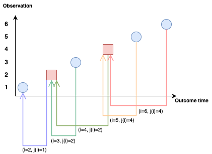
where \(CP\) is the set of comparable pairs defined by \(CP = \{(i, j) : t_i < t_j \wedge \delta_i = 1\}\). Given the number of pairs, the optimization problem quickly becomes difficult to solve with a very long runtime. To solve this problem Van Belle et al. (2011) found an efficient reduction that sorts observations in order of outcome time and then compares each data point \(i\) with the observation that has the next smallest survival time, skipping over censored observations, in maths: \(j(i) := \mathop{\mathrm{arg\,max}}_{j \in 1,...,n} \{t_j : t_j < t_i\}\). This is visualized in Figure 15.4 where six observations are sorted by outcome time from smallest (left) to largest (right). Starting from right to left, the first pair is made by matching the observation to the first uncensored outcome to the left, this continues to the end. In order for all observations to be used in the optimisation, the algorithm sets the first outcome to be uncensored hence observation \(2\) being compared to observation \(1\).
Using this reduction, the algorithm becomes
\[ \begin{aligned} & \min_{\boldsymbol{\beta}, \alpha, \boldsymbol{\xi}} \frac{1}{2}\|\boldsymbol{\beta}\|^2 + \gamma\sum_{i =1}^n \xi_i \\ & \textrm{subject to} \begin{dcases} g(\mathbf{x}_i) - g(\mathbf{x}_{j(i)}) & \geq t_i - t_{j(i)} - \xi_i \\ \xi_i & \geq 0 \end{dcases} \end{aligned} \]
\(\forall i = 1,...,n\). Note the updated right hand side of the constraint, which plays a similar role to the \(\epsilon\) parameter by allowing ‘mistakes’ in predictions without penalty.
Predictions for a new observation \(\mathbf{x}^*\) are calculated as,
\[ \hat{g}(\mathbf{x}^*) = \sum^n_{i=1} \mu_i(K(\mathbf{x}_i, \mathbf{x}^*) - K(\mathbf{x}_{j(i)}, \mathbf{x}^*)) + \alpha \]
Where \(\mu_i\) are again Lagrange multipliers.
15.2.3 Hybrid SSVMs
Finally, Van Belle et al. (2011) noted that the ranking algorithm could be updated to add the constraints of the regression model, thus providing a model that simultaneously optimizes for ranking whilst providing continuous values that can be interpreted as survival time predictions. This results in the hybrid SSVM with constraints \(\forall i = 1,...,n\):
\[ \begin{aligned} & \min_{\boldsymbol{\beta}, \alpha, \boldsymbol{\xi}, \boldsymbol{\xi}', \boldsymbol{\xi}^*} \frac{1}{2}\|\boldsymbol{\beta}\|^2 + \textcolor{CornflowerBlue}{\gamma\sum_{i =1}^n \xi_i} + \textcolor{Rhodamine}{C \sum^n_{i=1}(\xi_i' + \xi_i^*)} \\ & \textrm{subject to} \begin{dcases} \textcolor{CornflowerBlue}{g(\mathbf{x}_i) - g(\mathbf{x}_{j(i)})} & \textcolor{CornflowerBlue}{\geq t_i - t_{j(i)} - \xi_i} \\ \textcolor{Rhodamine}{g(\mathbf{x}_i)} & \textcolor{Rhodamine}{\leq t_i + \xi^*_i, i:\delta_i=1} \\ \textcolor{Rhodamine}{g(\mathbf{x}_i)} & \textcolor{Rhodamine}{\geq t_i - \xi'_i} \\ \textcolor{CornflowerBlue}{\xi_i}, \textcolor{Rhodamine}{\xi_i', \xi_i^*} & \geq 0 \\ \end{dcases} \end{aligned} \label{eq:surv_ssvmvb2} \]
The blue parts of the equation make up the ranking model and the red parts are the regression model. \(\gamma\) is the penalty associated with the regression method and \(C\) is the penalty associated with the ranking method. Setting \(\gamma = 0\) results in the regression SVM and \(C = 0\) results in the ranking SSVM. Hence, fitting the hybrid model and tuning these parameters is an efficient way to automatically detect which SSVM is best suited to a given task.
Once the model is fit, a prediction from given features \(\mathbf{x}^* \in \mathbb{R}^p\), can be made using the equation below, again with the ranking and regression contributions highlighted in blue and red respectively.
\[ \hat{g}(\mathbf{x}^*) = \sum^n_{i=1} \textcolor{CornflowerBlue}{\mu_i(K(\mathbf{x}_i, \mathbf{x}^*) - K(\mathbf{x}_{j(i)}, \mathbf{x}^*))} + \textcolor{Rhodamine}{\mu^*_i K(\mathbf{x}_i, \mathbf{x}^*) - \delta_i\mu_i'K(\mathbf{x}_i, \mathbf{x}^*)} + \alpha \]
where \(\mu_i, \mu_i^*, \mu_i'\) are Lagrange multipliers and \(K\) is a chosen kernel function, which may have further hyper-parameters to select or tune.