13 Classical Models
This page is a work in progress and major changes will be made over time.
TODO
- change chapter name (don’t use “classical”)
13.1 A Review of Classical Survival Models
This chapter provides a brief review of classical survival models before later chapters move on to machine learning models. ‘Classical’ models are defined with a very narrow scope in this book: low-complexity models that are either non-parametric or have parameters that can be fit with maximum likelihood estimation (or an equivalent method). In contrast, ‘machine learning’ (ML) models require more intensive model fitting procedures such as recursion or iteration. The classical models in this paper are fast to fit and highly interpretable, though can be inflexible and may make unreasonable assumptions. Whereas the ML models are more flexible with hyper-parameters however are computationally more intensive (both in terms of speed and storage), require tuning to produce ‘good’ results, and are often a ‘black-box’ with difficult interpretation.
As classical survival models have been studied extensively for decades, these are only discussed briefly here, primarily these are of interest as many of these models will be seen to influence machine learning extensions. The scope of the models discussed in this chapter is limited to the general book scope (?sec-surv-scope), i.e. single event with right-censoring and no competing-risks, though in some cases these are discussed.
There are several possible taxonomies for categorising statistical models, these include:
- Parametrisation Type: One of non-, semi-, or fully-parametric. \ Non-parametric models assume that the data distribution cannot be specified with a finite set of parameters. In contrast, fully-parametric models assume the distribution can be specified with a finite set of parameters. Semi-parametric models are a hybrid of the two and are formed of a finite set of parameters and an infinite-dimensional ‘nuisance’ parameter.
- Conditionality Type: One of unconditional or conditional. A conditional prediction is one that makes use of covariates in order to condition the prediction on each observation. Unconditional predictors, which are referred to below as ‘estimators’, ignore covariate data and make the same prediction for all individuals.
- Prediction Type: One of ranking, survival time, or distribution (Section 6.1).
Table 13.1 summarises the models discussed below into the taxonomies above for reference. Note that the Cox model is listed as predicting a continuous ranking, and not a survival distribution, which may appear inconsistent with other definitions. The reason for this is elaborated upon in Chapter 19. Though the predict-type taxonomy is favoured throughout this book, it is clearer to review classical models in increasing complexity, beginning with unconditional estimators before moving onto semi-parametric continuous ranking predictions, and finally conditional distribution predictors. The review is brief with mathematics limited to the model fundamentals but not including methods for parameter estimation. Also the review is limited to the ‘basic’ model specification and common extensions such as regularization are not discussed though they do exist for many of these models.
All classical models are highly transparent and accessible, with decades of research and many off-shelf implementations. Predictive performance of each model is briefly discussed as part of the review and then again in (R. E. B. Sonabend 2021).
| Model\(^1\) | Parametrisation\(^2\) | Prediction\(^3\) | Conditionality |
|---|---|---|---|
| Kaplan-Meier | Non | Distr. | Unconditional |
| Nelson-Aalen | Non | Distr. | Unconditional |
| Akritas | Non | Distr. | Conditional |
| Cox PH | Semi | Rank | Conditional |
| Parametric PH | Fully | Distr. | Conditional |
| Accelerated Failure Time | Fully | Distr. | Conditional |
| Proportional Odds | Fully | Distr. | Conditional |
| Flexible Spline | Fully | Distr. | Conditional |
* 1. All models are implemented in the \(\textsf{R}\) package \(\textbf{survival}\) (Therneau 2015) with the exception of flexible splines, implemented in \(\textbf{flexsurv}\) (Jackson 2016), and the Akritas estimator in \(\textbf{survivalmodels}\) (R. Sonabend 2020). * 2. Non = non-parametric, Semi = semi-parametric, Fully = fully-parametric. * 3. Distr. = distribution, Rank = ranking.
13.1.1 Non-Parametric Distribution Estimators
Unconditional Estimators
Unconditional non-parametric survival models assume no distribution for survival times and estimate the survival function using simple algorithms based on observed outcomes and no covariate data. The two most common methods are the Kaplan-Meier estimator (KaplanMeier1958?), which estimates the average survival function of a training dataset, and the Nelson-Aalen estimator (Aalen 1978; Nelson 1972), which estimates the average cumulative hazard function of a training dataset.
The Kaplan-Meier estimator of the survival function is given by \[ \hat{S}_{KM}(\tau|\mathcal{D}_{train}) = \prod_{t \in \mathcal{U}_O, t \leq \tau} \Big(1 - \frac{d_t}{n_t}\Big) \tag{13.1}\] As this estimate is so important in survival models, this book will always use the symbol \(\hat{S}_{KM}\) to refer to the Kaplan-Meier estimate of the average survival function fit on training data \((T_i, \Delta_i)\). Another valuable function is the Kaplan-Meier estimate of the average survival function of the censoring distribution, which is the same as above but estimated on \((T_i, 1 - \Delta_i)\), this will be denoted by \(\hat{G}_{KM}\).
The Nelson-Aalen estimator for the cumulative hazard function is given by \[ \hat{H}(\tau|\mathcal{D}_{train}) = \sum_{t \in \mathcal{U}_O, t \leq \tau} \frac{d_t}{n_t} \tag{13.2}\]
The primary advantage of these models is that they rely on heuristics from empirical outcomes only and don’t require any assumptions about the form of the data. To train the models they only require \((T_i,\Delta_i)\) and both return a prediction of \(\mathcal{S}\subseteq \operatorname{Distr}(\mathcal{T})\) ((box-task-surv?)). In addition, both simply account for censoring and can be utilised in fitting other models or to estimate unknown censoring distributions. The Kaplan-Meier and Nelson-Aalen estimators are both consistent estimators for the survival and cumulative hazard functions respectively.
Utilising the relationships provided in (Section 6.1), one could write the Nelson-Aalen estimator in terms of the survival function as \(\hat{S}_{NA} = \exp(-\hat{H}(\tau|\mathcal{D}_{train}))\). It has been demonstrated that \(\hat{S}_{NA}\) and \(\hat{S}_{KM}\) are asymptotically equivalent, but that \(\hat{S}_{NA}\) will provide larger estimates than \(\hat{S}_{KM}\) in smaller samples (Colosimo et al. 2002). In practice, the Kaplan-Meier is the most widely utilised non-parametric estimator in survival analysis and is the simplest estimator that yields consistent estimation of a survival distribution; it is therefore a natural, and commonly utilised, ‘baseline’ model (Binder and Schumacher 2008; Herrmann et al. 2021; Huang et al. 2020; Wang, Li, and Reddy 2019): estimators that other models should be ‘judged’ against to ascertain their overall performance (Chapter 7).
Not only can these estimators be used for analytical comparison, but they also provide intuitive methods for graphical calibration of models (Section 9.2). These models are never stuidied for prognosis directly but as baselines, components of complex models (Chapter 19), or graphical tools (Habibi et al. 2018; Jager et al. 2008; Moghimi-dehkordi et al. 2008). The reason for this is due to them having poor predictive performance as a result of omitting explanatory variables in fitting. Moreover, if the data follows a particular distribution, parametric methods will be more efficient (Wang, Li, and Reddy 2019).
Conditional Estimators
The Kaplan-Meier and Nelson-Aalen estimators are simple to compute and provide good estimates for the survival time distribution but in many cases they may be overly-simplistic. Conditional non-parametric estimators include the advantages described above (no assumptions about underlying data distribution) but also allow for conditioning the estimation on the covariates. This is particularly useful when estimating a censoring distribution that may depend on the data (Chapter 7). However predictive performance of conditional non-parametric estimators decreases as the number of covariates increases, and these models are especially poor when censoring is feature-dependent (Gerds and Schumacher 2006).
The most widely used conditional non-parametric estimator for survival analysis is the Akritas estimator (Akritas 1994) defined by \[ \hat{S}(\tau|X^*, \mathcal{D}_{train}, \lambda) = \prod_{j:T_j \leq \tau, \Delta_j = 1} \Big(1 - \frac{K(X^*, X_j|\lambda)}{\sum_{l = 1}^n K(X^*, X_l|\lambda)\mathbb{I}(T_l \geq T_j)}\Big) \] where \(K\) is a kernel function, usually \(K(x,y|\lambda) = \mathbb{I}(\lvert \hat{F}_X(x) - \hat{F}_X(y)\rvert < \lambda), \lambda \in (0, 1]\), \(\hat{F}_X\) is the empirical distribution function of the training data, \(X_1,...,X_n\), and \(\lambda\) is a hyper-parameter. The estimator can be interpreted as a conditional Kaplan-Meier estimator which is computed on a neighbourhood of subjects closest to \(X^*\) (Blanche, Dartigues, and Jacqmin-Gadda 2013). To account for tied survival times, the following adaptation of the estimator is utilised (Blanche, Dartigues, and Jacqmin-Gadda 2013)
\[ \hat{S}(\tau|X^*, \mathcal{D}_{train}, \lambda) = \prod_{t \in \mathcal{U}_O, t \leq \tau} \Big(1 - \frac{\sum^n_{j=1} K(X^*,X_j|\lambda)\mathbb{I}(T_j = t, \Delta_j = 1)}{\sum^n_{j=1} K(X^*,X_j|\lambda)\mathbb{I}(T_j \geq t)}\Big) \tag{13.3}\] If \(\lambda = 1\) then \(K(\cdot|\lambda) = 1\) and the estimator is identical to the Kaplan-Meier estimator.
The non-parametric nature of the model is highlighted in (Equation 13.3), in which both the fitting and predicting stages are combined into a single equation. A new observation, \(X^*\), is compared to its nearest neighbours from a training dataset, \(\mathcal{D}_{train}\), without a separated fitting procedure. One could consider splitting fitting and predicting in order to clearly separate between training and testing data. In this case, the fitting procedure is the estimation of \(\hat{F}_X\) on training data and the prediction is given by (Equation 13.3) with \(\hat{F}_X\) as an argument. This separated fit/predict method is implemented in \(\textbf{survivalmodels}\) (R. Sonabend 2020). As with other non-parametric estimators, the Akritas estimator can still be considered transparent and accessible. With respect to predictive performance, the Akritas estimator has more explanatory power than non-parametric estimators due to conditioning on covariates, however this is limited to a very small number of variables and therefore this estimator is still best placed as a conditional baseline.
13.1.2 Continuous Ranking and Semi-Parametric Models: Cox PH
The Cox Proportional Hazards (CPH) (Cox 1972), or Cox model, is likely the most widely known semi-parametric model and the most studied survival model (Habibi et al. 2018; Moghimi-dehkordi et al. 2008; Reid 1994; Wang, Li, and Reddy 2019). The Cox model assumes that the hazard for a subject is proportionally related to their explanatory variables, \(X_1,...,X_n\), via some baseline hazard that all subjects in a given dataset share (‘the PH assumption’). The hazard function in the Cox PH model is defined by \[ h(\tau|X_i)= h_0(\tau)\exp(X_i\beta) \] where \(h_0\) is the non-negative baseline hazard function and \(\beta = \beta_1,...,\beta_p\) where \(\beta_i \in \mathbb{R}\) are coefficients to be fit. Note the proportional hazards (PH) assumption can be seen as the estimated hazard, \(h(\tau|X_i)\), is directly proportional to the model covariates \(\exp(X_i\beta)\). Whilst a form is assumed for the ‘risk’ component of the model, \(\exp(X_i\beta)\), no assumptions are made about the distribution of \(h_0\), hence the model is semi-parametric.
The coefficients, \(\beta\), are estimated by maximum likelihood estimation of the ‘partial likelihood’ (Cox 1975), which only makes use of ordered event times and does not utilise all data available (hence being ‘partial’). The partial likelihood allows study of the informative \(\beta\)-parameters whilst ignoring the nuisance \(h_0\). The predicted linear predictor, \(\hat{\eta} := X^*\hat{\beta}\), can be computed from the estimated \(\hat{\beta}\) to provide a ranking prediction.
Inspection of the model is also useful without specifying the full hazard by interpreting the coefficients as ‘hazard ratios’. Let \(p = 1\) and \(\hat{\beta} \in \mathbb{R}\) and let \(X_i,X_j \in \mathbb{R}\) be the covariates of two training observations, then the hazard ratio for these observations is the ratio of their hazard functions, \[ \frac{h(\tau|X_i)}{h(\tau|X_j)} = \frac{h_0(\tau)\exp(X_i\hat{\beta})}{h_0(\tau)\exp(X_j\hat{\beta})} = \exp(\hat{\beta})^{X_i - X_j} \]
If \(\exp(\hat{\beta}) = 1\) then \(h(\tau|X_i) = h(\tau|X_j)\) and thus the covariate has no effect on the hazard. If \(\exp(\hat{\beta}) > 1\) then \(X_i > X_j \rightarrow h(\tau|X_i) > h(\tau|X_i)\) and therefore the covariate is positively correlated with the hazard (increases risk of event). Finally if \(\exp(\hat{\beta}) < 1\) then \(X_i > X_j \rightarrow h(\tau|X_i) < h(\tau|X_i)\) and the covariate is negatively correlated with the hazard (decreases risk of event).
Interpreting hazard ratios is known to be a challenge, especially by clinicians who require simple statistics to communicate to patients (Sashegyi and Ferry 2017; Spruance et al. 2004). For example the full interpretation of a hazard ratio of ‘2’ for binary covariate \(X\) would be: ‘assuming that the risk of death is constant at all time-points then the instantaneous risk of death is twice as high in a patient with \(X\) than without’. Simple conclusions are limited to stating if patients are at more or less risk than others in their cohort. Further disadvantages of the model also lie in its lack of real-world interpretabilitity, these include (Reid 1994):
- the PH assumption may not be realistic and the risk of event may not be constant over time;
- the estimated baseline hazard from a non-parametric estimator is a discrete step-function resulting in a discrete survival distribution prediction despite time being continuous; and
- the estimated baseline hazard will be constant after the last observed time-point in the training set (Gelfand et al. 2000).
Despite these disadvantages, the model has been demonstrated to have excellent predictive performance and routinely outperforms (or at least does not underperform) sophisticated ML models (Gensheimer and Narasimhan 2018; Luxhoj and Shyur 1997; Van Belle et al. 2011) (and (R. E. B. Sonabend 2021)). It’s simple form and wide popularity mean that it is also highly transparent and accessible.
The next class of models address some of the Cox model disadvantages by making assumptions about the baseline hazard.
13.1.3 Conditional Distribution Predictions: Parametric Linear Models
Parametric Proportional Hazards
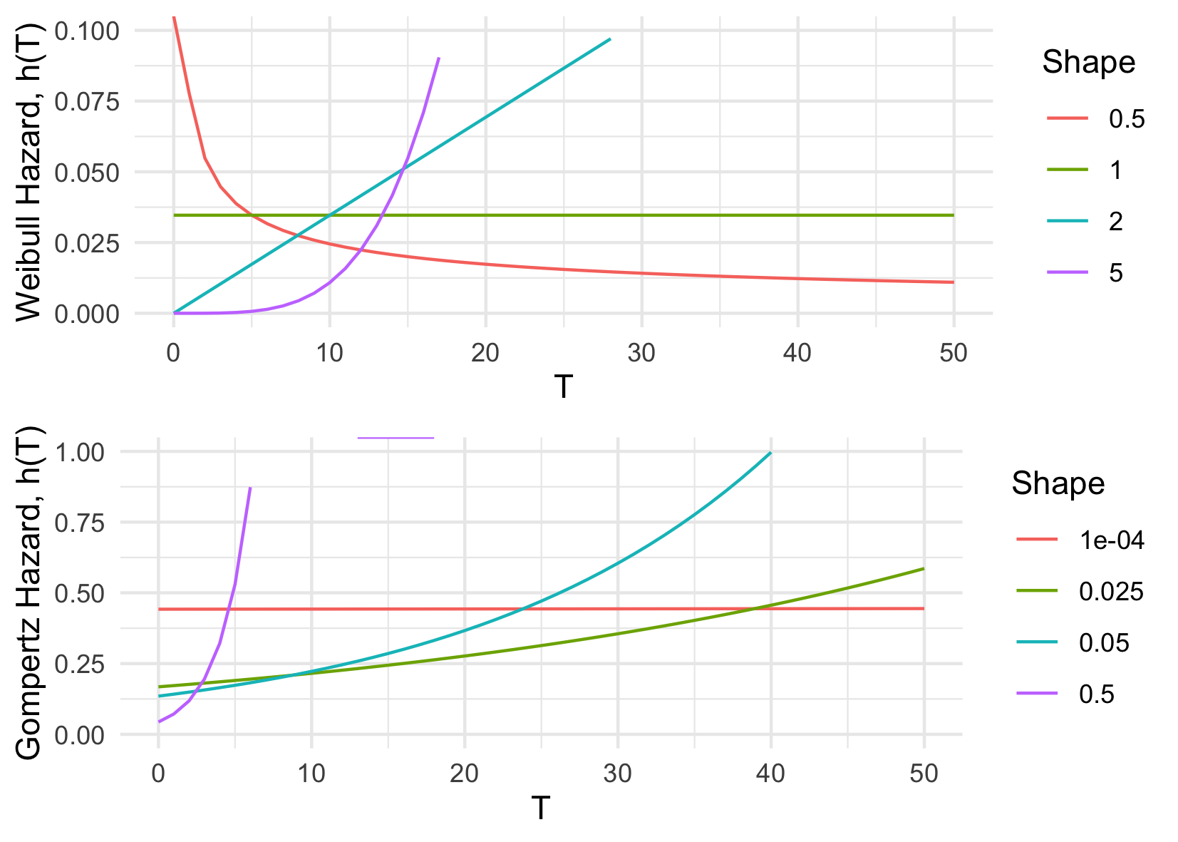
The CPH model can be extended to a fully parametric PH model by substituting the unknown baseline hazard, \(h_0\), for a particular parameterisation. Common choices for distributions are Exponential, Weibull and Gompertz (Kalbfleisch and Prentice 2011; Wang, Li, and Reddy 2019); their hazard functions are summarised in ((tab-survivaldists?)) along with the respective parametric PH model. Whilst an Exponential assumption leads to the simplest hazard function, which is constant over time, this is often not realistic in real-world applications. As such the Weibull or Gompertz distributions are often preferred. Moreover, when the shape parameter, \(\gamma\), is \(1\) in the Weibull distribution or \(0\) in the Gompertz distribution, their hazards reduce to a constant risk ((Figure 13.1)). As this model is fully parametric, the model parameters can be fit with maximum likelihood estimation, with the likelihood dependent on the chosen distribution.
| Distribution\(^1\) | \(h_0(\tau)^2\) | \(h(\tau|X_i)^3\) |
|---|---|---|
| \(\operatorname{Exp}(\lambda)\) | \(\lambda\) | \(\lambda\exp(X_i\beta)\) |
| \(\operatorname{Weibull}(\gamma, \lambda)\) | \(\lambda\gamma \tau^{\gamma-1}\) | \(\lambda\gamma \tau^{\gamma-1}\exp(X_i\beta)\) |
| \(\operatorname{Gompertz}(\gamma, \lambda)\) | \(\lambda \exp(\gamma \tau)\) | \(\lambda \exp(\gamma \tau)\exp(X_i\beta)\) |
* 1. Distribution choices for baseline hazard. \(\gamma,\lambda\) are shape and scale parameters respectively. * 2. Baseline hazard function, which is the (unconditional) hazard of the distribution. * 3. PH hazard function, \(h(\tau|X_i) = h_0(\tau)\exp(X_i\beta)\).
In the literature, the Weibull distribution tends to be favoured as the initial assumption for the survival distribution (Gensheimer and Narasimhan 2018; Habibi et al. 2018; Hielscher et al. 2010; R. and J. 1968; Rahman et al. 2017), though Gompertz is often tested in death-outcome models for its foundations in modelling human mortality (Gompertz 1825). There exist many tests for checking the goodness-of-model-fit (?sec-eval-insample) and the distribution choice can even be treated as a model hyper-parameter. Moreover it transpires that model inference and predictions are largely insensitive to the choice of distribution (Collett 2014; Reid 1994). In contrast to the Cox model, fully parametric PH models can predict absolutely continuous survival distributions, they do not treat the baseline hazard as a nuisance, and in general will result in more precise and interpretable predictions if the distribution is correctly specified (Reid 1994; Royston and Parmar 2002).
Whilst misspecification of the distribution tends not to affect predictions too greatly, PH models will generally perform worse when the PH assumption is not valid. PH models can be extended to include time-varying coefficients or model stratification (Cox 1972) but even with these adaptations the model may not reflect reality. For example, the predicted hazard in a PH model will be either monotonically increasing or decreasing but there are many scenarios where this is not realistic, such as when recovering from a major operation where risks tends to increase in the short-term before decreasing. Accelerated failure time models overcome this disadvantage and allow more flexible modelling, discussed next.
Accelerated Failure Time
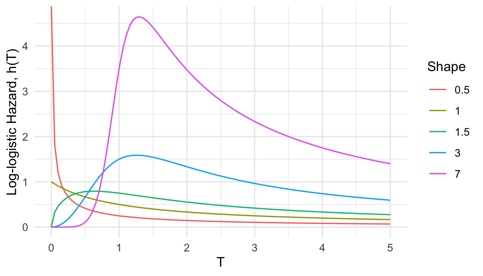
In contrast to the PH assumption, where a unit increase in a covariate is a multiplicative increase in the hazard rate, the Accelerated Failure Time (AFT) assumption means that a unit increase in a covariate results in an acceleration or deceleration towards death (expanded on below). The hazard representation of an AFT model demonstrates how the interpretation of covariates differs from PH models, \[ h(\tau|X_i)= h_0(\exp(-X_i\beta)\tau)\exp(-X_i\beta) \] where \(\beta = (\beta_1,...,\beta_p)\) are model coefficients. In contrast to PH models, the ‘risk’ component, \(\exp(-X_i\beta)\), is the exponential of the negative linear predictor and therefore an increase in a covariate value results in a decrease of the predicted hazard. This representation also highlights how AFT models are more flexible than PH as the predicted hazard can be non-monotonic. For example the hazard of the Log-logistic distribution ((Figure 13.2)) is highly flexible depending on chosen parameters. Not only can the AFT model offer a wider range of shapes for the hazard function but it is more interpretable. Whereas covariates in a PH model act on the hazard, in an AFT they act on time, which is most clearly seen in the log-linear representation, \[ \log Y_i = \mu + \alpha_1X_{i1} + \alpha_2X_{i2} + ... + \alpha_pX_{ip} + \sigma\epsilon_i \] where \(\mu\) and \(\sigma\) are location and scale parameters respectively, \(\alpha_1,...,\alpha_p\) are model coefficients, and \(\epsilon_i\) is a random error term. In this case a one unit increase in covariate \(X_{ij}\) means a \(\alpha_j\) increase in the logarithmic survival time. For example if \(\exp(X_i\alpha) = 0.5\) then \(i\) ‘ages’ at double the baseline ‘speed’. Or less abstractly if studying the time until death from cancer then \(\exp(X_i\alpha) = 0.5\) can be interpreted as ‘the entire process from developing tumours to metastasis and eventual death in subject \(i\) is twice as fast than the normal’, where ‘normal’ refers to the baseline when all covariates are \(0\).
Specifying a particular distribution for \(\epsilon_i\) yields a fully-parametric AFT model. Common distribution choices include Weibull, Exponential, Log-logistic, and Log-Normal (Kalbfleisch and Prentice 2011; Wang, Li, and Reddy 2019). The Buckley-James estimator (Buckley and James 1979) is a semi-parametric AFT model that non-parametrically estimates the distribution of the errors however this model has no theoretical justification and is rarely fit in practice (Wei 1992). The fully-parametric model has theoretical justifications, natural interpretability, and can often provide a better fit than a PH model, especially when the PH assumption is violated (Patel, Kay, and Rowell 2006; Qi 2009; Zare et al. 2015).
Proportional Odds
Proportional odds (PO) models (Bennett 1983) fit a proportional relationship between covariates and the odds of survival beyond a time \(\tau\), \[ O_i(\tau) = \frac{S_i(\tau)}{F_i(\tau)} = O_0(\tau)\exp(X_i\beta) \] where \(O_0\) is the baseline odds.
In this model, a unit increase in a covariate is a multiplicative increase in the odds of survival after a given time and the model can be interpreted as estimating the log-odds ratio. There is no simple closed form expression for the partial likelihood of the PO model and hence in practice a Log-logistic distribution is usually assumed for the baseline odds and the model is fit by maximum likelihood estimation on the full likelihood (Bennett 1983).
Perhaps the most useful feature of the model is convergence of hazard functions (Kirmani and Gupta 2001), which states \(h_i(\tau)/h_0(\tau) \rightarrow 1\) as \(\tau \rightarrow \infty\). This property accurately reflects real-world scenarios, for example if comparing chemotherapy treatment on advanced cancer survival rates, then it is expected that after a long period (say 10 years) the difference in risk between groups is likely to be negligible. This is in contrast to the PH model that assumes the hazard ratios are constant over time, which is rarely a reflection of reality.
In practice, the PO model is harder to fit and is less flexible than PH and AFT models, both of which can also produce odds ratios. This may be a reason for the lack of popularity of the PO model, in addition there is limited off-shelf implementations (Collett 2014). Despite PO models not being commonly utilised, they have formed useful components of neural networks (Section 17.1) and flexible parametric models (below).
Flexible Parametric Models – Splines
Royston-Parmar flexible parametric models (Royston and Parmar 2002) extend PH and PO models by estimating the baseline hazard with natural cubic splines. The model was designed to keep the form of the PH or PO methods but without the semi-parametric problem of estimating a baseline hazard that does not reflect reality (see above), or the parametric problem of misspecifying the survival distribution.
To provide an interpretable, informative and smooth hazard, natural cubic splines are fit in place of the baseline hazard. The crux of the method is to use splines to model time on a log-scale and to either estimate the log cumulative Hazard for PH models, \(\log H(\tau|X_i) = \log H_0(\tau) + X_i\beta\), or the log Odds for PO models, \(\log O(\tau|X_i) = \log O_0(\tau) + X_i\beta\), where \(\beta\) are model coefficients to fit, \(H_0\) is the baseline cumulative hazard function and \(O_0\) is the baseline odds function. For the flexible PH model, a Weibull distribution is the basis for the baseline distribution and a Log-logistic distribution for the baseline odds in the flexible PO model. \(\log H_0(\tau)\) and \(\log O_0(\tau)\) are estimated by natural cubic splines with coefficients fit by maximum likelihood estimation. The standard full likelihood is optimised, full details are not provided here. Between one and three internal knots are recommended for the splines and the placement of knots does not greatly impact upon the fitted model (Royston and Parmar 2002).
Advantages of the model include being: interpretable, flexible, can be fit with time-dependent covariates, and it returns a continuous function. Moreover many of the parameters, including the number and position of knots, are tunable, although Royston and Parmar advised against tuning and suggest often only one internal knot is required (Royston and Parmar 2002). A recent simulation study demonstrated that even with an increased number of knots (up to seven degrees of freedom), there was little bias in estimation of the survival and hazard functions (Bower et al. 2019). Despite its advantages, a 2018 review (Ng et al. 2018) found only twelve instances of published flexible parametric models since Royston and Parmar’s 2002 paper, perhaps because it is more complex to train, has a less intuitive fitting procedure than alternatives, and has limited off-shelf implementations; i.e. is less transparent and accessible than parametric alternatives.
The PH and AFT models are both very transparent and accessible, though require slightly more expert knowledge than the CPH in order to specify the ‘correct’ underlying probability distribution. Interestingly whilst there are many papers comparing PH and AFT models to one another using in-sample metrics (?sec-eval-insample) such as AIC (Georgousopoulou et al. 2015; Habibi et al. 2018; Moghimi-dehkordi et al. 2008; Zare et al. 2015), no benchmark experiments could be found for out-of-sample performance. PO and spline models are less transparent than PH and AFT models and are even less accessible, with very few implementations of either. No conclusions can be drawn about the predictive performance of PO or spline models due to a lack of suitable benchmark experiments.