17 Neural Networks
This page is a work in progress and major changes will be made over time.
17.1 Neural Networks
Before starting the survey on neural networks, first a comment about their transparency and accessibility. Neural networks are infamously difficult to interpret and train, with some calling building and training neural networks an ‘art’ (Hastie, Tibshirani, and Friedman 2001). As discussed in the introduction of this book, whilst neural networks are not transparent with respect to their predictions, they are transparent with respect to implementation. In fact the simplest form of neural network, as seen below, is no more complex than a simple linear model. With regard to accessibility, whilst it is true that defining a custom neural network architecture is complex and highly subjective, established models are implemented with a default architecture and are therefore accessible ‘off-shelf’.
17.1.1 Neural Networks for Regression
(Artificial) Neural networks (ANNs) are a class of model that fall within the greater paradigm of deep learning. The simplest form of ANN, a feed-forward single-hidden-layer network, is a relatively simple algorithm that relies on linear models, basic activation functions, and simple derivatives. A short introduction to feed-forward regression ANNs is provided to motivate the survival models. This focuses on single-hidden-layer models and increasing this to multiple hidden layers follows relatively simply.
The single hidden-layer network is defined through three equations \[\begin{align} & Z_m = \sigma(\alpha_{0m} + \alpha^T_mX_i), \quad m = 1,...,M \\ & T = \beta_{0k} + \beta_k^TZ, \quad k = 1,..,K \\ & g_k(X_i) = \phi_k(T) \end{align}\]
where \((X_1,...,X_n) \stackrel{i.i.d.}\sim X\) are the usual training data, \(\alpha_{0m}, \beta_0\) are bias parameters, and \(\theta = \{\alpha_m, \beta\}\) (\(m = 1,..,,M\)) are model weights where \(M\) is the number of hidden units. \(K\) is the number of classes in the output, which for regression is usually \(K = 1\). The function \(\phi\) is a ‘link’ or ‘activation function’, which transforms the predictions in order to provide an outcome of the correct return type; usually in regression, \(\phi(x) = x\). \(\sigma\) is the ‘activation function’, which transforms outputs from each layer. The \(\alpha_m\) parameters are often referred to as ‘activations’. Different activation functions may be used in each layer or the same used throughout, the choice is down to expert knowledge. Common activation functions seen in this section include the sigmoid function, \[ \sigma(v) = (1 + \exp(-v))^{-1} \] tanh function, \[ \sigma(v) = \frac{\exp(v) - \exp(-v)}{\exp(v) + \exp(-v)} \tag{17.1}\] and ReLU (Nair and Hinton 2010) \[ \sigma(v) = \max(0, v) \tag{17.2}\]
A single-hidden-layer model can also be expressed in a single equation, which highlights the relative simplicity of what may appear a complex algorithm.
\[ g_k(X_i) = \sigma_0(\beta_{k0} + \sum_{h=1}^H (\beta_{kh}\sigma_h (\beta_{h0} + \sum^M_{m=1} \beta_{hm}X_{i;m})) \tag{17.3}\] where \(H\) are the number of hidden units, \(\beta\) are the model weights, \(\sigma_h\) is the activation function in unit \(h\), also \(\sigma_0\) is the output unit activation, and \(X_{i;m}\) is the \(i\)th observation features in the \(m\)th hidden unit.
An example feed-forward single-hidden-layer regression ANN is displayed in (Figure 17.1). This model has 10 input units, 13 hidden units, and one output unit; two bias parameters are fit. The model is described as ‘feed-forward’ as there are no cycles in the node and information is passed forward from the input nodes (left) to the output node (right).
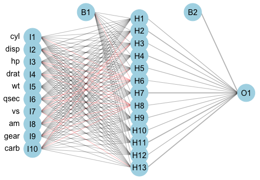
mtcars (Henderson and Velleman 1981) dataset using the \(\textbf{nnet}\) (N. Venables and D. Ripley 2002) package, and (Stasinopoulos et al. 2020) for plotting. Left column are input variables, I1-I10, second column are 13 hidden units, H1-H13, right column is single output variable, O1. B1 and B2 are bias parameters.
Back-Propagation
The model weights, \(\theta\), in this section are commonly fit by ‘back-propagation’ although this method is often considered inefficient compared to more recent advances. A brief pseudo-algorithm for the process is provided below.
Let \(L\) be a chosen loss function for model fitting, let \(\theta = (\alpha, \beta)\) be model weights, and let \(J \in \mathbb{N}_{> 0}\) be the number of iterations to train the model over. Then the back-propagation method is given by,
- For \(j = 1,...,J\): [] Forward Pass [i.] Fix weights \(\theta^{(j-1)}\). [ii.] Compute predictions \(\hat{Y} := \hat{g}^{(j)}_k(X_i|\theta^{(j-1)})\) with (Equation 17.3). [] Backward Pass [iii.] Calculate the gradients of the loss \(L(\hat{Y}|\mathcal{D}_{train})\). [] Update *[iv.] Update \(\alpha^{(r)}, \beta^{(r)}\) with gradient descent.
- End For
In regression, a common choice for \(L\) is the squared loss, \[ L(\hat{g}, \theta|\mathcal{D}_{train}) = \sum_{i=1}^n (Y_i - \hat{g}(X_i|\theta))^2 \] which may help illustrate how the training outcome, \((Y_1,...,Y_n) \stackrel{i.i.d.}\sim Y\), is utilised for model fitting.
Making Predictions
Once the model is fitted, predictions for new data follow by passing the testing data as inputs to the model with fitted weights,
\[ g_k(X^*) = \sigma_0(\hat{\beta}_{k0} + \sum_{h=1}^H (\hat{\beta}_{kh}\sigma_h (\hat{\beta}_{h0} + \sum^M_{m=1} \hat{\beta}_{hm}X^*_m)) \]
Hyper-Parameters
In practice, a regularization parameter, \(\lambda\), is usually added to the loss function in order to help avoid overfitting. This parameter has the effect of shrinking model weights towards zero and hence in the context of ANNs regularization is usually referred to as ‘weight decay’. The value of \(\lambda\) is one of three important hyper-parameters in all ANNs, the other two are: the range of values to simulate initial weights from, and the number of hidden units, \(M\).
The range of values for initial weights is usually not tuned but instead a consistent range is specified and the neural network is trained multiple times to account for randomness in initialization.
The regularization parameter and number of hidden units, \(M\), depend on each other and have a similar relationship to the learning rate and number of iterations in the GBMs (?sec-surv-ml-models-boost). Like the GBMs, it is simplest to set a high number of hidden units and then tune the regularization parameter (Bishop 2006; Hastie, Tibshirani, and Friedman 2001). Determining how many hidden layers to include, and how to connect them, is informed by expert knowledge and well beyond the scope of this book; decades of research has been required to derive sensible new configurations.
Training Batches
ANNs can either be trained using complete data, in batches, or online. This decision is usually data-driven and will affect the maximum number of iterations used to train the algorithm; as such this will also often be chosen by expert-knowledge and not empirical methods such as cross-validation.
Neural Terminology
Neural network terminology often reflects the structures of the brain. Therefore ANN units are referred to as nodes or neurons and sometimes the connections between neurons are referred to as synapses. Neurons are said to be ‘fired’ if they are ‘activated’. The simplest example of activating a neuron is with the Heaviside activation function with a threshold of \(0\): \(\sigma(v) = \mathbb{I}(v \geq 0)\). Then a node is activated and passes its output to the next layer if its value is positive, otherwise it contributes no value to the next layer.
17.1.2 Neural Networks for Survival Analysis
Surveying neural networks is a non-trivial task as there has been a long history in machine learning of publishing very specific data-driven neural networks with limited applications; this is also true in survival analysis. This does mean however that where limited developments for survival were made in other machine learning classes, ANN survival adaptations have been around for several decades. A review in 2000 by Schwarzer \(\textit{et al.}\) surveyed 43 ANNs for diagnosis and prognosis published in the first half of the 90s, however only up to ten of these are specifically for survival data. Of those, Schwarzer \(\textit{et al.}\) deemed three to be ‘na"ive applications to survival data’, and recommended for future research models developed by Liestl \(\textit{et al.}\) (1994) (Liestol, Andersen, and Andersen 1994), Faraggi and Simon (1995) (Faraggi and Simon 1995), and Biganzoli \(\textit{et al.}\) (1998) (E. Biganzoli et al. 1998).
This survey will not be as comprehensive as the 2000 survey, and nor has any survey since, although there have been several ANN reviews (B. D. Ripley and Ripley 2001; Huang et al. 2020a; Ohno-Machado 1996; Yang 2010; W. Zhu et al. 2020). ANNs are considered to be a black-box model, with interpretability decreasing steeply as the number of hidden layers and nodes increases. In terms of accessibility there have been relatively few open-source packages developed for survival ANNs; where these are available the focus has historically been in Python, with no \(\textsf{R}\) implementations. The new \(\textbf{survivalmodels}\) (R. Sonabend 2020) package, implements these Python models via \(\textbf{reticulate}\) (Ushey, Allaire, and Tang 2020). No recurrent neural netwoks are included in this survey though the survival models SRN (Oh et al. 2018) and RNN-Surv (Giunchiglia, Nemchenko, and Schaar 2018) are acknowledged.
This survey is made slightly more difficult as neural networks are often proposed for many different tasks, which are not necessarily clearly advertised in a paper’s title or abstract. For example, many papers claim to use neural networks for survival analysis and make comparisons to Cox models, whereas the task tends to be death at a particular (usually 5-year) time-point (classification) (Han et al. 2018; Lundin et al. 1999; B. D. Ripley and Ripley 2001; R. M. Ripley, Harris, and Tarassenko 1998; Huseyin Seker et al. 2002), which is often not made clear until mid-way through the paper. Reviews and surveys have also conflated these different tasks, for example a very recent review concluded superior performance of ANNs over Cox models, when in fact this is only in classification (Huang et al. 2020b) (RM2) {sec:car_reduxstrats_mistakes}. To clarify, this form of classification task does fall into the general field of survival analysis, but not the survival task ((box-task-surv?)). Therefore this is not a comment on the classification task but a reason for omitting these models from this survey.
Using ANNs for feature selection (often in gene expression data) and computer vision is also very common in survival analysis, and indeed it is in this area that most success has been seen (Bello et al. 2019; Chen, Ke, and Chiu 2014; Cui et al. 2020; Lao et al. 2017; McKinney et al. 2020; Rietschel, Yoon, and Schaar 2018; H. Seker et al. 2002; Zhang et al. 2020; X. Zhu, Yao, and Huang 2016), but these are again beyond the scope of this survey.
The key difference between neural networks is in their output layer, required data transformations, the model prediction, and the loss function used to fit the model. Therefore the following are discussed for each of the surveyed models: the loss function for training, \(L\), the model prediction type, \(\hat{g}\), and any required data transformation. Notation is continued from the previous surveys with the addition of \(\theta\) denoting model weights (which will be different for each model).
17.1.2.1 Probabilistic Survival Models
Unlike other classes of machine learning models, the focus in ANNs has been on probabilistic models. The vast majority make these predictions via reduction to binary classification \(\ref{sec:car_reduxes_r7}\). Whilst almost all of these networks implicitly reduce the problem to classification, most are not transparent in exactly how they do so and none provide clear or detailed interface points in implementation allowing for control over this reduction. Most importantly, the majority of these models do not detail how valid survival predictions are derived from the binary setting, which is not just a theoretical problem as some implementations, such as the Logistic-Hazard model in \(\textbf{pycox}\) (Kvamme 2018), have been observed to make survival predictions outside the range \([0,1]\). This is not a statement about the performance of models in this section but a remark about the lack of transparency across all probabilistic ANNs.
Many of these algorithms use an approach that formulate the Cox PH as a non-linear model and minimise the partial likelihood. These are referred to as ‘neural-Cox’ models and the earliest appears to have been developed by Faraggi and Simon (Faraggi and Simon 1995). All these models are technically composites that first predict a ranking, however they assume a PH form and in implementation they all appear to return a probabilistic prediction.
ANN-COX {#mod-anncox}\ Faraggi and Simon (Faraggi and Simon 1995) proposed a non-linear PH model \[ h(\tau|X_i,\theta) = h_0(\tau)\exp(\phi(X_i\beta)) \tag{17.4}\] where \(\phi\) is the sigmoid function and \(\theta = \{\beta\}\) are model weights. This model, ‘ANN-COX’, estimates the prediction functional, \(\hat{g}(X^*) = \phi(X^*\hat{\beta})\). The model is trained with the partial-likelihood function \[ L(\hat{g}, \theta|\mathcal{D}_{train}) = \prod_{i = 1}^n \frac{\exp(\sum^M_{m=1} \alpha_m\hat{g}_m(X^*))}{\sum_{j \in \mathcal{R}_{t_i}} \exp(\sum^M_{m=1} \alpha_m\hat{g}_m(X^*))} \] where \(\mathcal{R}_{t_i}\) is the risk group alive at \(t_i\); \(M\) is the number of hidden units; \(\hat{g}_m(X^*) = (1 + \exp(-X^*\hat{\beta}_m))^{-1}\); and \(\theta = \{\beta, \alpha\}\) are model weights.
The authors proposed a single hidden layer network, trained using back-propagation and weight optimisation with Newton-Raphson. This architecture did not outerperform a Cox PH (Faraggi and Simon 1995). Further adjustments including (now standard) pre-processing and hyper-parameter tuning did not improve the model performance (Mariani et al. 1997). Further independent studies demonstrated worse performance than the Cox model (Faraggi and Simon 1995; Xiang et al. 2000).
COX-NNET {#mod-coxnnet}\ COX-NNET (Ching, Zhu, and Garmire 2018) updates the ANN-COX by instead maximising the regularized partial log-likelihood \[ L(\hat{g}, \theta|\mathcal{D}_{train}, \lambda) = \sum^n_{i=1} \Delta_i \Big[\hat{g}(X_i) \ - \ \log\Big(\sum_{j \in \mathcal{R}_{t_i}} \exp(\hat{g}(X_j))\Big)\Big] + \lambda(\|\beta\|_2 + \|w\|_2) \] with weights \(\theta = (\beta, w)\) and where \(\hat{g}(X_i) = \sigma(wX_i + b)^T\beta\) for bias term \(b\), and activation function \(\sigma\); \(\sigma\) is chosen to be the tanh function ((Equation 17.1)). In addition to weight decay, dropout (Srivastava et al. 2014) is employed to prevent overfitting. Dropout can be thought of as a similar concept to the variable selection in random forests, as each node is randomly deactivated with probability \(p\), where \(p\) is a hyper-parameter to be tuned.
Independent simulation studies suggest that COX-NNET does not outperform the Cox PH (Michael F. Gensheimer and Narasimhan 2019).
DeepSurv {#mod-deepsurv}\ DeepSurv (J. L. Katzman et al. 2018) extends these models to deep learning with multiple hidden layers. The chosen error function is the average negative log-partial-likelihood with weight decay \[ L(\hat{g}, \theta|\mathcal{D}_{train}, \lambda) = -\frac{1}{n^*} \sum_{i = 1}^n \Delta_i \Big[ \Big(\hat{g}(X_i) - \log \sum_{j \in \mathcal{R}_{t_i})} \exp(\hat{g}(X_j)\Big)\Big] + \lambda\|\theta\|^2_2 \] where \(n^* := \sum^n_{i=1} \mathbb{I}(\Delta_i = 1)\) is the number of uncensored observations and \(\hat{g}(X_i) = \phi(X_i|\theta)\) is the same prediction object as the ANN-COX. State-of-the-art methods are used for data pre-processing and model training. The model architecture uses a combination of fully-connected and dropout layers. Benchmark experiments by the authors indicate that DeepSurv can outperform the Cox PH in ranking tasks (J. Katzman et al. 2016; J. L. Katzman et al. 2018) although independent experiments do not confirm this (Zhao and Feng 2020).
*Cox-Time** {#mod-coxtime}\ Kvamme \(\textit{et al.}\) (Kvamme, Borgan, and Scheel 2019) build on these models by allowing time-varying effects. The loss function to minimise, with regularization, is given by \[ L(\hat{g}, \theta|\mathcal{D}_{train}, \lambda) = \frac{1}{n} \sum_{i:\Delta_i = 1} \log\Big(\sum_{j \in \mathcal{R}_{t_i}} \exp[\hat{g}(X_j,T_i) - \hat{g}(X_i, T_i)]\Big) + \lambda \sum_{i:\Delta_i=1}\sum_{j \in \mathcal{R}_{t_i}} |\hat{g}(X_j,T_i)| \] where \(\hat{g}= \hat{g}_1,...,\hat{g}_n\) is the same non-linear predictor but with a time interaction and \(\lambda\) is the regularization parameter. The model is trained with stochastic gradient descent and the risk set, \(\mathcal{R}_{t_i}\), in the equation above is instead reduced to batches, as opposed to the complete dataset. ReLU activations (Nair and Hinton 2010) and dropout are employed in training. Benchmark experiments indicate good performance of Cox-Time, though no formal statistical comparisons are provided and hence no comment about general performance can be made.
ANN-CDP {#mod-anncdp}\ One of the earliest ANNs that was noted by Schwarzer \(\textit{et al.}\) (Schwarzer, Vach, and Schumacher 2010) was developed by Liestl \(\textit{et al.}\) (Liestol, Andersen, and Andersen 1994) and predicts conditional death probabilities (hence ‘ANN-CDP’). The model first partitions the continuous survival times into disjoint intervals \(\mathcal{I}_k, k = 1,...,m\) such that \(\mathcal{I}_k\) is the interval \((t_{k-1}, t_k]\). The model then studies the logistic Cox model (proportional odds) (Cox 1972) given by \[ \frac{p_k(\mathbf{x})}{q_k(\mathbf{x})} = \exp(\eta + \theta_k) \] where \(p_k = 1-q_k\), \(\theta_k = \log(p_k(0)/q_k(0))\) for some baseline probability of survival, \(q_k(0)\), to be estimated; \(\eta\) is the usual linear predictor, and \(q_k = P(T \geq T_k | T \geq T_{k-1})\) is the conditional survival probability at time \(T_k\) given survival at time \(T_{k-1}\) for \(k = 1,...,K\) total time intervals. A logistic activation function is used to predict \(\hat{g}(X^*) = \phi(\eta + \theta_k)\), which provides an estimate for \(\hat{p}_k\).
The model is trained on discrete censoring indicators \(D_{ki}\) such that \(D_{ki} = 1\) if individual \(i\) dies in interval \(\mathcal{I}_k\) and \(0\) otherwise. Then with \(K\) output nodes and maximum likelihood estimation to find the model parameters, \(\hat{\eta}\), the final prediction provides an estimate for the conditional death probabilities \(\hat{p}_k\). The negative log-likelihood to optimise is given by \[ L(\hat{g}, \theta|\mathcal{D}_{train}) = \sum^n_{i=1}\sum^{m_i}_{k=1} [D_{ki}\log(\hat{p}_k(X_i)) + (1-D_{ki})\log(\hat{q}_k(X_i))] \] where \(m_i\) is the number of intervals in which observation \(i\) is not censored.
Liestl \(\textit{et al.}\){} discuss different weighting options and how they correspond to the PH assumption. In the most generalised case, a weight-decay type regularization is applied to the model weights given by \[ \alpha \sum_l \sum_k (w_{kl} - w_{k-1,l})^2 \] where \(w\) are weights, and \(\alpha\) is a hyper-parameter to be tuned, which can be used alongside standard weight decay. This corresponds to penalizing deviations from proportionality thus creating a model with approximate proportionality. The authors also suggest the possibility of fixing the weights to be equal in some nodes and different in others; equal weights strictly enforces the proportionality assumption. Their simulations found that removing the proportionality assumption completely, or strictly enforcing it, gave inferior results. Comparing their model to a standard Cox PH resulted in a ‘better’ negative log-likelihood, however this is not a precise evaluation metric and an independent simulation would be preferred. Finally Listl \(\textit{et al.}\) included a warning `‘The flexibility is, however, obtained at unquestionable costs: many parameters, difficult interpretation of the parameters and a slow numerical procedure’’ (Liestol, Andersen, and Andersen 1994).
PLANN {#mod-plann}\ Biganzoli \(\textit{et al.}\) (1998) (E. Biganzoli et al. 1998) studied the same proportional-odds model as the ANN-CDP (Liestol, Andersen, and Andersen 1994). Their model utilises partial logistic regression (Efron 1988) with added hidden nodes, hence ‘PLANN’. Unlike ANN-CDP, PLANN predicts a smoothed hazard function by using smoothing splines. The continuous time outcome is again discretised into disjoint intervals \(t_m, m = 1,...,M\). At each time-interval, \(t_m\), the number of events, \(d_m\), and number of subjects at risk, \(n_m\), can be used to calculate the discrete hazard function, \[ \hat{h}_m = \frac{d_m}{n_m}, m = 1,...,M \tag{17.5}\] This quantity is used as the target to train the neural network. The survival function is then estimated by the Kaplan-Meier type estimator, \[ \hat{S}(\tau) = \prod_{m:t_m \leq \tau} (1 - \hat{h}_m) \tag{17.6}\]
The model is fit by employing one of the more ‘usual’ survival reduction strategies in which an observation’s survival time is treated as a covariate in the model (Tutz and Schmid 2016). As this model uses discrete time, the survival time is discretised into one of the \(M\) intervals. This approach removes the proportional odds constraint as interaction effects between time and covariates can be modelled (as time-updated covariates). Again the model makes predictions at a given time \(m\), \(\phi(\theta_m + \eta)\), where \(\eta\) is the usual linear predictor, \(\theta\) is the baseline proportional odds hazard \(\theta_m = \log(h_m(0)/(1-h_m(0))\). The logistic activation provides estimates for the discrete hazard, \[ h_m(X_i) = \frac{\exp(\theta_m + \hat{\eta})}{1 + \exp(\theta_m + \hat{\eta})} \] which is smoothed with cubic splines (Efron 1988) that require tuning.
A cross-entropy error function is used for training \[ L(\hat{h}, \theta|\mathcal{D}_{train}, a) = - \sum^M_{m = 1} \Big[\hat{h}_m \log \Big(\frac{h_l(X_i, a_l)}{\hat{h}_m}\Big) + (1 - \hat{h}_m) \log \Big(\frac{1 - h_l(X_i, a_l)}{1 - \hat{h}_m}\Big)\Big]n_m \] where \(h_l(X_i, a_l)\) is the discrete hazard \(h_l\) with smoothing at mid-points \(a_l\). Weight decay can be applied and the authors suggest \(\lambda \approx 0.01-0.1\) (E. Biganzoli et al. 1998), though they make use of an AIC type criterion instead of cross-validation.
This model makes smoothed hazard predictions at a given time-point, \(\tau\), by including \(\tau\) in the input covariates \(X_i\). Therefore the model first requires transformation of the input data by replicating all observations and replacing the single survival indicator \(\Delta_i\), with a time-dependent indicator \(D_{ik}\), the same approach as in ANN-CDP. Further developments have extended the PLANN to Bayesian modelling, and for competing risks (E. M. Biganzoli, Ambrogi, and Boracchi 2009).
No formal comparison is made to simpler model classes. The authors recommend ANNs primarily for exploration, feature selection, and understanding underlying patterns in the data (E. M. Biganzoli, Ambrogi, and Boracchi 2009).
Nnet-survival {#mod-nnetsurvival}\ Aspects of the PLANN algorithm have been generalised into discrete-time survival algorithms in several papers (Michael F. Gensheimer and Narasimhan 2019; Kvamme2019?; Mani et al. 1999; Street 1998). Various estimates have been derived for transforming the input data to a discrete hazard or survival function. Though only one is considered here as it is the most modern and has a natural interpretation as the ‘usual’ Kaplan-Meier estimator for the survival function. Others by Street (1998) (Street 1998) and Mani (1999) (Mani et al. 1999) are acknowledged. The discrete hazard estimator (Equation 17.5), \(\hat{h}\), is estimated and these values are used as the targets for the ANN. For the error function, the mean negative log-likelihood for discrete time (Kvamme2019?) is minimised to estimate \(\hat{h}\), \[ \begin{split} L(\hat{h}, \theta|\mathcal{D}_{train}) = -\frac{1}{n} \sum^n_{i=1}\sum^{k(T_i)}_{j=1} (\mathbb{I}(T_i = \tau_j, \Delta_i = 1) \log[\hat{h}_i(\tau_j)] \ + \\ (1-\mathbb{I}(T_i = \tau_j, \Delta_i = 1))\log(1 - \hat{h}_i(\tau_j))) \end{split} \] where \(k(T_i)\) is the time-interval index in which observation \(i\) dies/is censored, \(\tau_j\) is the \(j\)th discrete time-interval, and the prediction of \(\hat{h}\) is obtained via \[ \hat{h}(\tau_j|\mathcal{D}_{train}) = [1 + \exp(-\hat{g}_j(\mathcal{D}_{train}))]^{-1} \] where \(\hat{g}_j\) is the \(j\)th output for \(j = 1,...,m\) discrete time intervals. The number of units in the output layer for these models corresponds to the number of discrete-time intervals. Deciding the width of the time-intervals is an additional hyper-parameter to consider.
Gensheimer and Narasimhan’s ‘Nnet-survival’ (Michael F. Gensheimer and Narasimhan 2019) has two different implementations. The first assumes a PH form and predicts the linear predictor in the final layer, which can then be composed to a distribution. Their second ‘flexible’ approach instead predicts the log-odds of survival in each node, which are then converted to a conditional probability of survival, \(1 - h_j\), in a given interval using the sigmoid activation function. The full survival function can be derived with (Equation 17.6). The model has been demonstrated not to outperform the Cox PH with respect to Harrell’s C or the Graf (Brier) score (Michael F. Gensheimer and Narasimhan 2019).
PC-Hazard {#mod-pchazard}\ Kvamme and Borgan deviate from nnet-survival in their ‘PC-Hazard’ (Kvamme2019?) by first considering a discrete-time approach with a softmax activation function influenced by multi-class classification. They expand upon this by studying a piecewise constant hazard function in continuous time and defining the mean negative log-likelihood as \[ L(\hat{g}, \theta|\mathcal{D}_{train}) = -\frac{1}{n} \sum^n_{i=1} \Big(\Delta_i X_i\log\tilde{\eta}_{k(T_i)} - X_i\tilde{\eta}_{k(T_i)}\rho(T_i) - \sum^{k(T_i)-1}_{j=1} \tilde{\eta}_jX_i\Big) \] where \(k(T_i)\) and \(\tau_i\) is the same as defined above, \(\rho(t) = \frac{t - \tau_{k(t)-1}}{\Delta\tau_{k(t)}}\), \(\Delta\tau_j = \tau_j - \tau_{j-1}\), and \(\tilde{\eta}_j := \log(1 + \exp(\hat{g}_j(X_i))\) where again \(\hat{g}_j\) is the \(j\)th output for \(j = 1,...,m\) discrete time intervals. Once the weights have been estimated, the predicted survival function is given by \[ \hat{S}(\tau, X^*|\mathcal{D}_{train}) = \exp(-X^*\tilde{\eta}_{k(\tau)}\rho(\tau)) \prod^{k(\tau)-1}_{j=1} \exp(-\tilde{\eta}_j(X^*)) \] Benchmark experiments indicate similar performance to nnet-survival (Kvamme2019?), an unsurprising result given their implementations are identical with the exception of the loss function (Kvamme2019?), which is also similar for both models. A key result found that varying values for interval width lead to significant differences and therefore should be carefully tuned.
DNNSurv {#mod-dnnsurv}\ A very recent (pre-print) approach (Zhao and Feng 2020) instead first computes ‘pseudo-survival probabilities’ and uses these to train a regression ANN with sigmoid activation and squared error loss. These pseudo-probabilities are computed using a jackknife-style estimator given by \[ \tilde{S}_{ij}(T_{j+1}, \mathcal{R}_{t_j}) = n_j\hat{S}(T_{j+1}|\mathcal{R}_{t_j}) - (n_j - 1)\hat{S}^{-i}(T_{j+1}|\mathcal{R}_{t_j}) \] where \(\hat{S}\) is the IPCW weighted Kaplan-Meier estimator (defined below) for risk set \(\mathcal{R}_{t_j}\), \(\hat{S}^{-i}\) is the Kaplan-Meier estimator for all observations in \(\mathcal{R}_{t_j}\) excluding observation \(i\), and \(n_j := |\mathcal{R}_{t_j}|\). The IPCW weighted Kaplan-Meier estimate is found via the IPCW Nelson-Aalen estimator, \[ \hat{H}(\tau|\mathcal{D}_{train}) = \sum^n_{i=1} \int^\tau_0 \frac{\mathbb{I}(T_i \leq u, \Delta_i = 1)\hat{W}_i(u)}{\sum^n_{j=1} \mathbb{I}(T_j \geq u) \hat{W}_j(u)} \ du \] where \(\hat{W}_i,\hat{W}_j\) are subject specific IPC weights.
In their simulation studies, they found no improvement over other proposed neural networks. Arguably the most interesting outcome of their paper are comparisons of multiple survival ANNs at specific time-points, evaluated with C-index and Brier score. Their results indicate identical performance from all models. They also provide further evidence of neural networks not outperforming a Cox PH when the PH assumption is valid. However, in their non-PH dataset, DNNSurv appears to outperform the Cox model (no formal tests are provided). Data is replicated similarly to previous models except that no special indicator separates censoring and death, this is assumed to be handled by the IPCW pseudo probabilities.
DeepHit {#mod-deephit}\ DeepHit (Lee et al. 2018) was originally built to accommodate competing risks, but only the non-competing case is discussed here (Kvamme, Borgan, and Scheel 2019). The model builds on previous approaches by discretising the continuous time outcome, and makes use of a composite loss. It has the advantage of making no parametric assumptions and directly predicts the probability of failure in each time-interval (which again correspond to different terminal nodes), i.e. \(\hat{g}(\tau_k|\mathcal{D}_{test}) = \hat{P}(T^* = \tau_k|X^*)\) where again \(\tau_k, k = 1,...,K\) are the distinct time intervals. The estimated survival function is found with \(\hat{S}(\tau_K|X^*) = 1 - \sum^K_{k = 1} \hat{g}_i(\tau_k|X^*)\). ReLU activations were used in all fully connected layers and a softmax activation in the final layer. The losses in the composite error function are given by \[ L_1(\hat{g}, \theta|\mathcal{D}_{train}) = -\sum^N_{i=1} [\Delta_i \log(\hat{g}_i(T_i)) + (1-\Delta_i)\log(\hat{S}_i(T_i))] \] and \[ L_2(\hat{g}, \theta|\mathcal{D}_{train}, \sigma) = \sum_{i \neq j} \Delta_i \mathbb{I}(T_i < T_j) \sigma(\hat{S}_i(T_i), \hat{S}_j(T_i)) \] for some convex loss function \(\sigma\) and where \(\hat{g}_i(t) = \hat{g}(t|X_i)\). Again these can be seen to be a cross-entropy loss and a ranking loss. Benchmark experiments demonstrate the model outperforming the Cox PH and RSFs (Lee et al. 2018) with respect to separation, and an independent experiment supports these findings (Kvamme, Borgan, and Scheel 2019). However, the same independent study demonstrated worse performance than a Cox PH with respect to the integrated Brier score (Graf et al. 1999).
17.1.2.2 Deterministic Survival Models
Whilst the vast majority of survival ANNs have focused on probabilistic predictions (often via ranking), a few have also tackled the deterministic or ‘hybrid’ problem.
RankDeepSurv {#mod-rankdeepsurv}\ Jing \(\textit{et al.}\) (Jing et al. 2019) observed the past two decades of research in survival ANNs and then published a completely novel solution, RankDeepSurv, which makes predictions for the survival time \(\hat{T} = (\hat{T}_1,...,\hat{T}_n)\). They proposed a composite loss function \[ L(\hat{T}, \theta|\mathcal{D}_{train}, \alpha,\gamma,\lambda) = \alpha L_1(\hat{T},T,\Delta) + \gamma L_2(\hat{T},T,\Delta) + \lambda\|\theta\|^2_2 \] where \(\theta\) are the model weights, \(\alpha,\gamma \in \mathbb{R}_{>0}\), \(\lambda\) is the shrinkage parameter, by a slight abuse of notation \(T = (T_1,...,T_n)\) and \(\Delta = (\Delta_1,...,\Delta_n)\), and \[ L_1(\hat{T}, \theta|\mathcal{D}_{train}) = \frac{1}{n} \sum_{\{i: I(i) = 1\}} (\hat{T}_i - T_i)^2; \quad I(i) = \begin{cases} 1, & \Delta_i = 1 \cup (\Delta_i = 0 \cap \hat{T}_i \leq T_i) \\ 0, & \text{otherwise} \end{cases} \] \[ L_2(\hat{T}, \theta|\mathcal{D}_{train}) = \frac{1}{n}\sum^n_{\{i,j : I(i,j) = 1\}} [(T_j - T_i) - (\hat{T}_j - \hat{T}_i)]^2; \quad I(i,j) = \begin{cases} 1, & T_j - T_i > \hat{T}_j - \hat{T}_i \\ 0, & \text{otherwise} \end{cases} \] where \(\hat{T}_i\) is the predicted survival time for observation \(i\). A clear contrast can be made between these loss functions and the constraints used in SSVM-Hybrid (Van Belle et al. 2011) (Section 15.2). \(L_1\) is the squared second constraint in \(\ref{eq:surv_ssvmvb2}\) and \(L_2\) is the squared first constraint in \(\ref{eq:surv_ssvmvb2}\). However \(L_1\) in RankDeepSurv discards the squared error difference for all censored observations when the prediction is lower than the observed survival time; which is problematic as if someone is censored at time \(T_i\) then it is guaranteed that their true survival time is greater than \(T_i\) (this constraint may be more sensible if the inequality were reversed). An advantage to this loss is, like the SSVM-Hybrid, it enables a survival time interpretation for a ranking optimised model; however these ‘survival times’ should be interpreted with care.
The authors propose a model architecture with several fully connected layers with the ELU (Clevert, Unterthiner, and Hochreiter 2015) activation function and a single dropout layer. Determining the success of this model is not straightforward. The authors claim superiority of RankDeepSurv over Cox PH, DeepSurv, and RSFs however this is an unclear comparison (RM2) {sec:car_reduxstrats_mistakes} that requires independent study.
17.1.3 Conclusions
There have been many advances in neural networks for survival analysis. It is not possible to review all proposed survival neural networks without diverting too far from the book scope. This survey of ANNs should demonstrate two points: firstly that the vast majority (if not all) of survival ANNs are reduction models that either find a way around censoring via imputation or discretisation of time-intervals, or by focusing on partial likelihoods only; secondly that no survival ANN is fully accessible or transparent.
Despite ANNs being highly performant in other areas of supervised learning, there is strong evidence that the survival ANNs above are inferior to a Cox PH when the data follows the PH assumption or when variables are linearly related (Michael F. Gensheimer and Narasimhan 2018; Luxhoj and Shyur 1997; Ohno-Machado 1997; Puddu and Menotti 2012; Xiang et al. 2000; Yang 2010; Yasodhara, Bhat, and Goldenberg 2018; Zhao and Feng 2020). There are not enough experiments to make conclusions in the case when the data is non-PH. Experiments in (R. E. B. Sonabend 2021) support the finding that survival ANNs are not performant.
There is evidence that many papers introducing neural networks do not utilise proper methods of comparison or evaluation (Király, Mateen, and Sonabend 2018) and in conducting this survey, these findings are further supported. Many papers made claims of being ‘superior’ to the Cox model based on unfair comparisons (RM2){sec:car_reduxstrats_mistakes} or miscommunicating (or misinterpreting) results (e.g. (Fotso 2018)). At this stage, it does not seem possible to make any conclusions about the effectiveness of neural networks in survival analysis. Moreover, even the authors of these models have pointed out problems with transparency (E. M. Biganzoli, Ambrogi, and Boracchi 2009; Liestol, Andersen, and Andersen 1994), which was further highlighted by Schwarzer \(\textit{et al.}\) (Schwarzer, Vach, and Schumacher 2010).
Finally, accessibility of neural networks is also problematic. Many papers do not release their code and instead just state their networks architecture and available packages. In theory, this is enough to build the models however this does not guarantee the reproducibility that is usually expected. For users with a technical background and good coding ability, many of the models above could be implemented in one of the neural network packages in \(\textsf{R}\), such as \(\textbf{nnet}\) (N. Venables and D. Ripley 2002) and \(\textbf{neuralnet}\) (Fritsch, Guenther, and N. Wright 2019); though in practice the only package that does contain these models, \(\textbf{survivalmodels}\), does not directly implement the models in \(\textsf{R}\) (which is much slower than Python) but provides a method for interfacing the Python implementations in \(\textbf{pycox}\) (Kvamme 2018).