14 Random Forests
This page is a work in progress and major changes will be made over time.
14.1 Random Forests for Regression
Random forests are a composite algorithm built by fitting many simpler component models, decision trees, and then averaging the results of predictions from these trees. Decision trees are first briefly introduced before the key ‘bagging’ algorithm, which creates the random forest. Woodland terminology is used throughout this chapter.
Decision Trees
Decision trees are a common model class in machine learning and have the advantage of being (relatively) simple to implement and highly interpretable. A decision tree takes a set of inputs and a given splitting rule in order to create a series of splits, or branches, in the tree that culminates in a final leaf, or terminal node. Each terminal node has a corresponding prediction, which for regression is usually the sample mean of the training outcome data. This is made clearer by example, (Figure 14.1) demonstrates a decision tree predicting the miles per gallon (mpg) of a car from the mtcars (Henderson and Velleman 1981) dataset. With this tree a new prediction is made by feeding the input variables from the top to the bottom, for example given new data, \(x = \{`wt` = 3, `disp` = 250\}\), then in the first split the right branch is taken as wt \(= 3 > 2.32\) and in the second split the left branch is taken as disp \(= 250 \leq 258\), therefore the new data point ‘lands’ in the final leaf and is predicted to have an mpg of \(20.8\). This value of \(20.8\) arises as the sample mean of mpg for the \(11\) (which can be seen in the box) observations in the training data who were sorted into this terminal node. Algorithmically, as splits are always binary, predictions are simply a series of conditional logical statements.
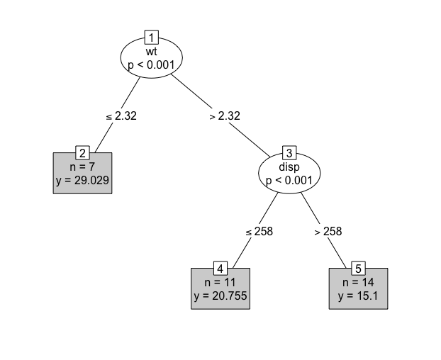
mtcars (Henderson and Velleman 1981) dataset and the \(\textbf{party}\) (Hothorn, Hornik, and Zeileis 2006) package. Ovals are leaves, which indicate the variable that is being split. Edges are branches, which indicate the cut-off at which the variable is split. Rectangles are terminal nodes and include information about the number of training observations in the node and the terminal node prediction.
Splitting Rules
Precisely how the splits are derived and which variables are utilised is determined by the splitting rule. In regression, the most common splitting rule is to select the cut-off for a given variable that minimises the mean squared error in each hypothetical resultant leaf. The goal is to find the variable and cutoff that leads to the greatest difference between the two resultant leaves and thus the maximal homogeneity within each leaf. For all decision tree and random forest algorithms going forward, let \(L\) denote some leaf, then let \(L_{xy}, L_x, L_y\) respectively be the set of observations, features, and outcomes in leaf \(L\). Let \(L_{y;i}\) be the \(i\)th outcome in \(L_y\) and finally let \(L_{\bar{y}} = \frac{1}{n} \sum^{n}_{i = 1} L_{y;i}\). To simplify notation, \(i \in L\) is taken to be equivalent to \(i \in \{i: X_i \in L_X\}\), i.e. the indices of the observations in leaf \(L\).
Let \(c \in \mathbb{R}\) be some cutoff parameter and let \(L^a_{xy}(j,c) := \{(X_i,Y_i)|X_{ij} < c, i = 1,...,n\}, L^b_{xy}(j,c) = \{(X_i,Y_i)|X_{ij} \geq c, i = 1,...,n\}\) be the two leaves containing the set of observations resulting from partitioning variable \(j\) at cutoff \(c\). Then a split is determined by finding the arguments, \((j^*,c^*)\) that minimise the sum of the mean squared errors (MSE) in both leaves (James et al. 2013), \[ (j^*, c^*) = \mathop{\mathrm{arg\,min}}_{j, c} \sum_{y \in L^a_{y}(j,c)} (y - L^a_{\bar{Y}}(j,c))^2 + \sum_{y \in L^b_{y}(j,c)} (y - L^b_{\bar{Y}}(j,c))^2 \tag{14.1}\]
This method is repeated from the first branch of the tree down to the very last such that observations are included in a given leaf \(L\) if they satisfy all conditions from all previous branches; features may be considered multiple times in the growing process. This is an intuitive method as minimising the above sum results in the set of observations within each individual leaf being as similar as possible, thus as an observation is passed down the tree, it becomes more similar to the subsequent leaves, eventually landing in a leaf containing homogeneous observations. Controlling how many variables to consider at each split and how many splits to make are determined by hyper-parameter tuning.
Decision trees are a powerful method for high-dimensional data as only a small sample of variables will be used for growing a tree, and therefore they are also useful for variable importance by identifying which variables were utilised in growth (other importance methods are also available). Decision trees are also highly interpretable, as demonstrated by (Figure 14.1). The recursive pseudo-algorithm in ((alg-dt-fit?)) demonstrates the simplicity in growing a decision tree (again methods such as pruning are omitted).
Stopping Rules
The ‘stopping rule’ in ((alg-dt-fit?)) is usually a condition on the number of observations in each leaf such that leaves will continue to be split until some minimum number of observations has been reached in a leaf. Other conditions may be on the ‘depth’ of the tree, which corresponds to the number of levels of splitting, for example the tree in (Figure 14.1) has a depth of \(2\) (the first level is not counted).
Random Forests
Despite being more interpretable than other machine learning methods, decision trees usually have poor predictive performance, high variance and are not robust to changes in the data. As such, random forests are preferred to improve prediction accuracy and decrease variance. Random forests utilise bootstrap aggregation, or bagging (Breiman 1996), to aggregate many decision trees. A pseudo fitting algorithm is given in ((alg-rsf-fit?)).
Prediction from a random forest follows by making predictions from the individual trees and aggregating the results by some function \(\sigma\) ((alg-rsf-pred?)); \(\sigma\) is usually the sample mean for regression,
\[ \hat{g}(X^*) = \sigma(\hat{g}_1(X^*),...,\hat{g}_B(X^*)) = \frac{1}{B} \sum^B_{b=1} \hat{g}_b(X^*) \]
where \(\hat{g}_b(X^*)\) is the terminal node prediction from the \(b\)th tree and \(B\) are the total number of grown trees ($B$' is commonly used instead of\(N\)’ to note the relation to bootstrapped data).
Usually many (hundreds or thousands) trees are grown, which makes random forests robust to changes in data and ‘confident’ about individual predictions. Other advantages include having several tunable hyper-parameters, including: the number of trees to grow, the number of variables to include in a single tree, the splitting rule, and the minimum terminal node size. Machine learning models with many hyper-parameters, tend to perform better than other models as they can be fine-tuned to the data, which is why complex deep learning models are often the best performing. Although as a caveat: too many parameters can lead to over-fitting and tuning many parameters can take a long time and be highly intensive. Random forests lose the interpretability of decision trees and are considered ‘black-box’ models as individual predictions cannot be easily scrutinised.
14.2 Random Survival Forests
Unlike other machine learning methods that may require complex changes to underlying algorithms, random forests can be relatively simply adapted to random survival forests by updating the splitting rules and terminal node predictions to those that can handle censoring and can make survival predictions. This chapter is therefore focused on outlining different choices of splitting rules and terminal node predictions, which can then be flexibly combined into different models.
14.2.1 Splitting Rules
Survival trees and RSFs have been studied for the past four decades and whilst the amount of splitting rules to appear could be considered `‘numerous’’ (Bou-Hamad, Larocque, and Ben-Ameur 2011), only two broad classes are commonly utilised and implemented (H. Ishwaran and Kogalur 2018; Pölsterl 2020; Therneau and Atkinson 2019; Wright and Ziegler 2017). The first class rely on hypothesis tests, and primarily the log-rank test, to maximise dissimilarity between splits, the second class utilises likelihood-based measures. The first is discussed in more detail as this is common in practice and is relatively straightforward to implement and understand, moreover it has been demonstrated to outperform other splitting rules (Bou-Hamad, Larocque, and Ben-Ameur 2011). Likelihood rules are more complex and require assumptions that may not be realistic, these are discussed briefly.
Hypothesis Tests
The log-rank test statistic has been widely utilised as the ‘natural’ splitting-rule for survival analysis (Ciampi et al. 1986; B. H. Ishwaran et al. 2008; LeBlanc and Crowley 1993; Segal 1988). The log-rank test compares the survival distributions of two groups and has the null-hypothesis that both groups have the same underlying risk of (immediate) death, i.e. identical hazard functions.
Let \(L^A\) and \(L^B\) be two leaves then using the notation above let \(h^A,h^B\) be the (true) hazard functions derived from the observations in the two leaves respectively. The log-rank hypothesis test is given by \(H_0: h^A = h^B\) with test statistic (Segal 1988), \[ LR(L^A) = \frac{\sum_{\tau \in \mathcal{U}_D} (d^A_{\tau} - e^A_{\tau})}{\sqrt{\sum_{\tau \in \mathcal{U}_D} v_\tau^A}} \]
where \(d^A_{\tau}\) is the observed number of deaths in leaf \(A\) at \(\tau\), \[ d^A_{\tau} := \sum_{i \in L^A} \mathbb{I}(T_i = \tau, \Delta_i = 1) \]
\(e^A_{\tau}\) is the expected number of deaths in leaf \(A\) at \(\tau\), \[ e^A_{\tau} := \frac{n_\tau^A d_\tau}{n_\tau} \]
and \(v^A_\tau\) is the variance of the number of deaths in leaf \(A\) at \(\tau\), \[ v^A_{\tau} := e^A_{\tau} \Big(\frac{n_\tau - d_\tau}{n_\tau}\Big)\Big(\frac{n_\tau - n^A_\tau}{n_\tau - 1}\Big) \]
where \(\mathcal{U}_D\) is the set of unique death times across the data (in both leaves), \ \(n_\tau = \sum_i \mathbb{I}(T_i \geq \tau)\) is the number of observations at risk at \(\tau\) in both leaves, \ \(n_\tau^A = \sum_{i \in L^A} \mathbb{I}(T_i \geq \tau)\) is the number of observations at risk at \(\tau\) in leaf A, and \ \(d_\tau = \sum_i \mathbb{I}(T_i = \tau, \Delta_i = 1)\) is the number of deaths at \(\tau\) in both leaves.
Intuitively these results follow as the number of deaths in a leaf is distributed according to \(\operatorname{Hyper}(n^A_\tau,n_\tau,d_\tau)\). The same statistic results if \(L^B\) is instead considered. ((alg-dt-fit?)) follows for fitting decision trees with the log-rank splitting rule, \(SR\), to be maximised.
The higher the log-rank statistic, the greater the dissimilarity between the two groups, thereby making it a sensible splitting rule for survival, moreover it has been shown that it works well for splitting censored data (LeBlanc and Crowley 1993). When censoring is highly dependent on the outcome, the log-rank statistic does not perform well and is biased (Bland and Altman 2004), which tends to be true of the majority of survival models. Additionally, the log-rank test requires no knowledge about the shape of the survival curves or distribution of the outcomes in either group (Bland and Altman 2004), making it ideal for an automated process that requires no user intervention.
The log-rank score rule (Hothorn and Lausen 2003) is a standardized version of the log-rank rule that could be considered as a splitting rule, though simulation studies have demonstrated non-significant predictive performance when comparing the two (B. H. Ishwaran et al. 2008).
Alternative dissimiliarity measures and tests have also been suggested as splitting rules, including modified Kolmogorov-Smirnov test and Gehan-Wilcoxon tests (Ciampi et al. 1988). Simulation studies have demonstrated that both of these may have higher power and produce ‘better’ results than the log-rank statistic (Fleming et al. 1980). Despite this, these do not appear to be in common usage and no implementation could be found that include these.
### Likelihood Based Rules {.unnumbered .unlisted} Likelihood ratio statistics, or deviance based splitting rules, assume a certain model form and thereby an assumption about the data. This may be viewed as an advantageous strategy, as it could arguably increase interpretability, or a disadvantage as it places restrictions on the data. For survival models, a full-likelihood can be estimated with a Cox form by estimating the cumulative hazard function (LeBlanc and Crowley 1992). LeBlanc and Crowley (1992) (LeBlanc and Crowley 1992) advocate for selecting the optimal split by maximising the full PH likelihood, assuming the cumulative hazard function, \(H\), is known, \[ \mathcal{L}:= \prod_{m = 1}^M \prod_{i \in L^m} h_m(T_i)^{\Delta_i} \exp(-H_m(T_i)) \]
where \(M\) is the total number of terminal nodes, \(h_m\) and \(H_m\) are the (true) hazard and cumulative hazard functions in the \(m\)th node, and again \(L^m\) is the set of observations in terminal node \(m\). Estimation of \(h_m\) and \(H_m\) are described with the associated terminal node prediction below.
The primary advantage of this method is that any off-shelf regression software with a likelihood splitting rule can be utilised without any further adaptation to model fitting by supplying this likelihood with required estimates. However the additional costs of computing these estimates may outweigh the benefits once the likelihood has been calculated, and this could be why only one implementation of this method has been found (Bou-Hamad, Larocque, and Ben-Ameur 2011; Therneau and Atkinson 2019).
Other Splitting Rules
As well as likelihood and log-rank spitting rules, other papers have studied comparison of residuals (Therneau, Grambsch, and Fleming 1990), scoring rules (H. Ishwaran and Kogalur 2018), and distance metrics (Gordon and Olshen 1985). These splitting rules work similarly to the mean squared error in the regression setting, in which the score should be minimised across both leaves. The choice of splitting rule is usually data-dependent and can be treated as a hyper-parameter for tuning. However, if there is a clear goal in prediction, then the choice of splitting rule can be informed by the prediction type. For example, if the goal is to maximise separation, then a log-rank splitting rule to maximise homogeneity in terminal nodes is a natural starting point. Whereas if the goal is to estimate the linear predictor of a Cox PH model, then a likelihood splitting rule with a Cox form may be more sensible.
14.2.2 Terminal Node Prediction
Only two terminal node predictions appear in common usage.
Predict: Ranking
Terminal node ranking predictions for survival trees and forests have been limited to those that use a likelihood-based splitting rule and assume a PH model form (H. Ishwaran et al. 2004; LeBlanc and Crowley 1992). In model fitting the likelihood splitting rule model attempts to fit the (theoretical) PH model \(h_m(\tau) = h_0(\tau)\theta_m\) for \(m \in 1,...,M\) where \(M\) is the total number of terminal nodes and \(\theta_m\) is a parameter to estimate. The model returns predictions for \(\exp(\hat{\theta}_m)\) where \(\hat{\theta}_m\) is the estimate of \(\theta_m\). This is estimated via an iterative procedure in which in iteration \(j+1\), \(\hat{\theta}_m^{j+1}\) is estimated by \[ \hat{\theta}_m^{j+1} = \frac{\sum_{i \in L^m} \Delta_i}{\sum_{i \in L^m} \hat{H}^j_0(T_i)} \]
where as before \(L^m\) is the set of observations in leaf \(m\) and \[ \hat{H}^{j}_0(\tau) = \frac{\sum_{i:T_i \leq \tau} \Delta_i}{\sum_{m = 1}^M\sum_{\{i:i \in \mathcal{R}_\tau \cap L^a\}} \hat{\theta}^{j}_m} \]
which is repeated until some stopping criterion is reached. The same cumulative hazard is estimated for all nodes however \(\hat{\theta}_m\) varies across nodes. This method lends itself naturally to a composition to a full distribution (Chapter 19) as it assumes a PH form and separately estimates the cumulative hazard and relative risk (?sec-surv-ml-models-ranfor-nov), though no implementation of this composition could be found.
Predict: Survival Distribution
The most common terminal node prediction appears to be predicting the survival distribution by estimating the survival function, using the Kaplan-Meier or Nelson-Aalen estimators, on the sample in the terminal node (Hothorn et al. 2004; B. H. Ishwaran et al. 2008; LeBlanc and Crowley 1993; Segal 1988). Estimating a survival function by a non-parametric estimator is a natural choice for terminal node prediction as these are natural ‘baselines’ in survival, similarly to taking the sample mean in regression. The prediction for SDTs is straightforward, the non-parametric estimator is fit on all observations in each of the terminal nodes. This is adapted to RSFs by bagging the estimator across all decision trees (Hothorn et al. 2004). Using the Nelson-Aalen estimator as an example, let \(m\) be a terminal node in an SDT, then the terminal node prediction is given by,
\[ \hat{H}_m(\tau) = \sum_{\{i: i \in L^m \cap T_i \leq \tau\}} \frac{d_i}{n_i} \tag{14.2}\] where \(d_i\) and \(n_i\) are the number of events and observations at risk at time \(T_i\) in terminal node \(m\). Ishwaran (B. H. Ishwaran et al. 2008) defined the bootstrapped Nelson-Aalen estimator as
\[ \hat{H}_{Boot}(\tau) = \frac{1}{B} \sum^B_{b=1} \hat{H}_{m, b}(\tau), \quad m \in 1,...,M \tag{14.3}\]
where \(B\) is the total number of bootstrapped estimators, \(M\) is the number of terminal nodes, and \(\hat{H}_{m,b}\) is the cumulative hazard for the \(m\)th terminal node in the \(b\)th tree. The bootstrapped Kaplan-Meier estimator is calculated analogously. More generally these can be considered as a uniform mixture of \(B\) distributions (Chapter 19).
All implemented RSFs can now be summarised into the following five algorithms:
RRT {#mod-rrt}\ LeBlanc and Crowley’s (1992) (LeBlanc and Crowley 1992) survival decision tree uses a deviance splitting rule with a terminal node ranking prediction, which assumes a PH model form. These ‘relative risk trees’ (RRTs) are implemented in the package \(\textbf{rpart}\) (Therneau and Atkinson 2019). This model is considered the least accessible and transparent of all discussed in this section as: few implementations exist, it requires assumptions that may not be realistic, and predictions are harder to interpret than other models. Predictive performance of the model is expected to be worse than RSFs as this is a decision tree; this is confirmed in (Sonabend 2021).
RRF {#mod-rrf}\ Ishwaran \(\textit{et al.}\) (2004) (H. Ishwaran et al. 2004) proposed a random forest framework for the relative risk trees, which makes a slight adaptation and applies the iteration of the terminal node prediction after the tree is grown as opposed to during the growing process. No implementation for these ‘relative risk forests’ (RRFs) could be found or any usage in the literature.
RSDF-DEV {#mod-rsdfdev}\ Hothorn \(\textit{et al.}\) (2004) (Hothorn et al. 2004) expanded upon the RRT by introducing a bagging composition thus creating a random forest with a deviance splitting rule, again assuming a PH form. However the ranking prediction is altered to be a bootstrapped Kaplan-Meier prediction in the terminal node. This is implemented in \(\textbf{ipred}\) (Peters and Hothorn 2019). This model improves upon the accessibility and transparency of the RRT by providing a more straightforward and interpretable terminal node prediction. However, as this is a decision tree, predictive performance is again expected to be worse than the RSFs.
RSCIFF {#mod-rsciff}\ Hothorn \(\textit{et al.}\) (Hothorn et al. 2005) studied a conditional inference framework in order to predict log-survival time. In this case the splitting rule is based on an IPC weighted loss function, which allows implementation by off-shelf classical random forests. The terminal node predictions are a weighted average of the log-survival times in the node where weighting is determined by the Kaplan-Meier estimate of the censoring distribution. This ‘random survival conditional inference framework forest’ (RSCIFF) is implemented in \(\textbf{party}\) (Hothorn, Hornik, and Zeileis 2006) and \(\textbf{partykit}\) (Hothorn and Zeileis 2015), which additionally includes a distribution terminal node prediction via the bootstrapped Kaplan-Meier estimator. The survival tree analogue (SDCIFT) is implemented in the same packages. Implementation of the RSCIFF is complex, which is likely why all implementations (in the above packages) are by the same authors. The complexity of conditional inference forests may also be the reason why several reviews, including this one, mention (or completely omit) RSCIFFs but do not include any comprehensive details that explain the fitting procedure (Bou-Hamad, Larocque, and Ben-Ameur 2011; Wang and Li 2017). In this regard, it is hard to claim that RSCIFFs are transparent or accessible. Moreover, the authors of the model state that random conditional inference forests are for `‘expert user[s] only and [their] current state is rather experimental’’ (Hothorn and Zeileis 2015). Finally, with respect to model performance, there is evidence that they can outperform RSDFs (below) dependent on the data type (Nasejje et al. 2017) however no benchmark experiment could be found that compared them to other models.
RSDF-STAT {#mod-rsdfstat}\ Finally Ishwaran \(\textit{et al.}\) (2008) (B. H. Ishwaran et al. 2008) proposed the most general form of RSFs with a choice of hypothesis tests (log-rank and log-rank score) and survival measure (Brier, concordance) splitting rules, and a bootstrapped Nelson-Aalen terminal node prediction. These are implemented in \(\textbf{randomForestSRC}\) (H. Ishwaran and Kogalur 2018) and \(\textbf{ranger}\) (Wright and Ziegler 2017). There are several implementations of these models across programming languages, and extensive details for the fitting and predicting procedures, which makes them very accessible. The models utilise a standard random forest framework, which makes them transparent and familiar to those without expert Survival knowledge. Moreover they have been proven to perform well in benchmark experiments, especially on high-dimensional data (Herrmann et al. 2021; Spooner et al. 2020).