19 Reductions
This page is a work in progress and major changes will be made over time.
In this chapter, composition and reduction are formally introduced, defined and demonstrated within survival analysis. Neither of these are novel concepts in general or in survival, with several applications already seen earlier when reviewing models (particularly in neural networks), however a lack of formalisation has led to much repeated work and at times questionable applications (Section 17.1). The primary purpose of this chapter is to formalise composition and reduction for survival and to unify references and strategies for future use. These strategies are introduced in the context of minimal ‘workflows’ and graphical ‘pipelines’ in order to maximise their generalisability. The pipelines discussed in this chapter are implemented in mlr3proba.
A workflow is a generic term given to a series of sequential operations. For example a standard ML workflow is fit/predict/evaluate, which means a model is fit, predictions are made, and these are evaluated. In this book, a pipeline is the name given to a concrete workflow. Section 19.1 demonstrates how pipelines are represented in this book.
Composition (Section 19.2) is a general process in which an object is built (or composed) from other objects and parameters. Reduction (Section 19.3) is a closely related concept that utilises composition in order to transform one problem into another. Concrete strategies for composition and reduction are detailed in sections Section 19.4 and Section 19.5.
Notation and Terminology
The notation introduced in Chapter 4 is recapped for use in this chapter: the generative survival template for the survival setting is given by \((X,T,\Delta,Y,C) \ t.v.i. \ \mathcal{X}\times \mathcal{T}\times \{0,1\}\times \mathcal{T}\times \mathcal{T}\) where \(\mathcal{X}\subseteq \mathbb{R}^p\) and \(\mathcal{T}\subseteq \mathbb{R}_{\geq 0}\), where \(C,Y\) are unobservable, \(T := \min\{Y,C\}\), and \(\Delta = \mathbb{I}(Y = T)\). Random survival data is given by \((X_i,T_i,\Delta_i,Y_i,C_i) \stackrel{i.i.d.}\sim(X,T,\Delta,Y,C)\). Usually data will instead be presented as a training dataset, \(\mathcal{D}_{train}= \{(X_1,T_1,\Delta_1),...,(X_n,T_n,\Delta_n)\}\) where \((X_i,T_i,\Delta_i) \stackrel{i.i.d.}\sim(X,T,\Delta)\), and some test data \(\mathcal{D}_{test}= (X^*,T^*,\Delta^*) \sim (X,T,\Delta)\).
For regression models the generative template is given by \((X,Y)\) t.v.i. \(\mathcal{X}\subseteq \mathbb{R}^p\) and \(Y \subseteq \mathbb{R}\). As with the survival setting, a regression training set is given by \(\{(X_1,Y_1),...,(X_n,Y_n)\}\) where \((X_i,Y_i) \stackrel{i.i.d.}\sim(X,Y)\) and some test data \((X^*,Y^*) \sim (X,Y)\).
19.1 Representing Pipelines
Before introducing concrete composition and reduction algorithms, this section briefly demonstrates how these pipelines will be represented in this book.
Pipelines are represented by graphs designed in the following way: all are drawn with operations progressing sequentially from left to right; graphs are comprised of nodes (or ‘vertices’) and arrows (or ‘directed edges’); a rounded rectangular node represents a process such as a function or model fitting/predicting; a (regular) rectangular node represents objects such as data or hyper-parameters. Output from rounded nodes are sometimes explicitly drawn but when omitted the output from the node is the input to the next.
These features are demonstrated in ?fig-car-example. Say \(y = 2\) and \(a = 2\), then: data is provided (\(y = 2\)) and passed to the shift function (\(f(x)=x + 2)\), the output of this function (\(y=4\)) is passed directly to the next \((h(x|a)=x^a)\), this function requires a parameter which is also input (\(a = 2\)), finally the resulting output is returned (\(y^*=16\)). Programmatically, \(a = 2\) would be a hyper-parameter that is stored and passed to the required function when the function is called.
This pipeline is represented as a pseudo-algorithm in (alg-car-ex?), though of course is overly complicated and in practice one would just code \((y+2)^\wedge a\).
19.2 Introduction to Composition
This section introduces composition, defines a taxonomy for describing compositors (Section 19.2.1), and provides some motivating examples of composition in survival analysis (Section 19.2.2).
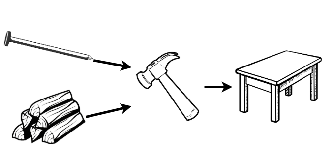
In the simplest definition, a model (be it mathematical, computational, machine learning, etc.) is called a composite model if it is built of two or more constituent parts. This can be simplest defined in terms of objects. Just as objects in the real-world can be combined in some way, so can mathematical objects. The exact ‘combining’ process (or ‘compositor’) depends on the specific composition, so too do the inputs and outputs. By example, a wooden table can be thought of as a composite object (Figure 19.1). The inputs are wood and nails, the combining process is hammering (assuming the wood is pre-chopped), and the output is a surface for eating. In mathematics, this process is mirrored. Take the example of a shifted linear regression model. This is defined by a linear regression model, \(f(x) = \beta_0 + x\beta_1\), a shifting parameter, \(\alpha\), and a compositor \(g(x|\alpha) = f(x) + \alpha\). Mathematically this example is overly trivial as this could be directly modelled with \(f(x) = \alpha + \beta_0 + x\beta_1\), but algorithmically there is a difference. The composite model \(g\), is defined by first fitting the linear regression model, \(f\), and then applying a shift, \(\alpha\); as opposed to fitting a directly shifted model.
Why Composition?
Tables tend to be better surfaces for eating your dinner than bundles of wood. Or in modelling terms, it is well-known that ensemble methods (e.g. random forests) will generally outperform their components (e.g. decision trees). All ensemble methods are composite models and this demonstrates one of the key use-cases of composition: improved predictive performance. The second key use-case is reduction, which is fully discussed in Section 19.3. Section 19.2.2 motivates composition in survival analysis by demonstrating how it is already prevalent but requires formalisation to make compositions more transparent and accessible.
Composite Model vs. Sub-models
A bundle of wood and nails is not a table and \(1,000\) decision trees are not a random forest, both require a compositor. The compositor in a composite model combines the components into a single model. Considering a composite model as a single model enables the hyper-parameters of the compositor and the component model(s) to be efficiently tuned whilst being evaluated as a single model. This further allows the composite to be compared to other models, including its own components, which is required to justify complexity instead of parsimony in model building (?sec-eval-why-why).
19.2.1 Taxonomy of Compositors
Just as there are an infinite number of ways to make a table, composition can come in infinite forms. However there are relatively few categories that these can be grouped into. Two primary taxonomies are identified here. The first is the ‘composition type’ and relates to the number of objects composed:
[i)] i. Single-Object Composition (SOC) – This form of composition either makes use of parameters or a transformation to alter a single object. The shifted linear regression model above is one example of this, another is given in Section 19.4.3. i. Multi-Object Composition (MOC) – In contrast, this form of composition combines multiple objects into a single one. Both examples in Section 19.2.2 are multi-object compositions.
The second grouping is the ‘composition level’ and determines at what ‘level’ the composition takes place:
[i)] i. Prediction Composition – This applies at the level of predictions; the component models could be forgotten at this point. Predictions may be combined from multiple models (MOC) or transformed from a single model (SOC). Both examples in Section 19.2.2 are prediction compositions. i. Task Composition – This occurs when one task (e.g. regression) is transformed to one or more others (e.g. classification), therefore always SOC. This is seen mainly in the context of reduction (Section 19.3). i. Model Composition – This is commonly seen in the context of wrappers (Section 19.5.1.4), in which one model is contained within another. i. Data Composition – This is transformation of training/testing data types, which occurs at the first stage of every pipeline.
19.2.2 Motivation for Composition
Two examples are provided below to demonstrate common uses of composition in survival analysis and to motivate the compositions introduced in Section 19.4.
Example 1: Cox Proportional Hazards
Common implementations of well-known models can themselves be viewed as composite models, the Cox PH is the most prominent example in survival analysis. Recall the model defined by
\[ h(\tau|X_i) = h_0(\tau)\exp(\beta X_i) \] where \(h_0\) is the baseline hazard and \(\beta\) are the model coefficients.
This can be seen as a composite model as Cox defines the model in two stages (Cox 1972): first fitting the \(\beta\)-coefficients using the partial likelihood and then by suggesting an estimate for the baseline distribution. This first stage produces a linear predictor return type (Section 6.1) and the second stage returns a survival distribution prediction. Therefore the Cox model for linear predictions is a single (non-composite) model, however when used to make distribution predictions then it is a composite. Cox implicitly describes the model as a composite by writing ‘’alternative simpler procedures would be worth having’’ (Cox 1972), which implies a decision in fitting (a key feature of composition). This composition is formalised in Section 19.4.1 as a general pipeline . The Cox model utilises the pipeline with a PH form and Kaplan-Meier baseline.
Example 2: Random Survival Forests
Fully discussed in Chapter 14, random survival forests are composed from many individual decision trees via a prediction composition algorithm ((alg-rsf-pred?)). In general, random forests perform better than their component decision trees, which tends to be true of all ensemble methods. Aggregation of predictions in survival analysis requires slightly more care than other fields due to the multiple prediction types, however this is still possible and is formalised in Section 19.4.4.
19.3 Introduction to Reduction
This section introduces reduction, motivates its use in survival analysis (Section 19.3.1), details an abstract reduction pipeline and defines the difference between a complete/incomplete reduction (Section 19.3.2), and outlines some common mistakes that have been observed in the literature when applying reduction (Section 19.3.3).
Reduction is a concept found across disciplines with varying definitions. This report uses the Langford definition: reduction is ‘’a complex problem decomposed into simpler subproblems so that a solution to the subproblems gives a solution to the complex problem’’ (Langford et al. 2016). Generalisation (or induction) is a common real-world use of reduction, for example sampling a subset of a population in order to estimate population-level results. The true answer (population-level values) may not always be found in this way but very good approximations can be made with simpler sub-problems (sub-sampling).
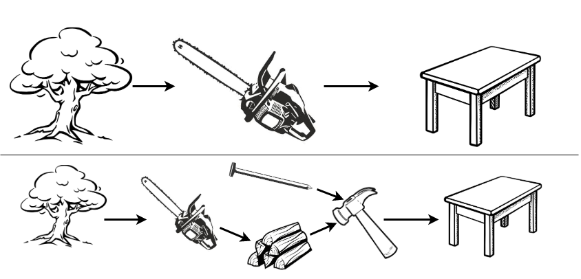
Reductions are workflows that utilise composition. By including hyper-parameters, even complex reduction strategies can remain relatively flexible. To illustrate reduction by example, recall the table-building example (Section 19.2) in which the task of interest is to acquire a table. The most direct but complex solution is to fell a tree and directly saw it into a table (Figure 19.2, top), clearly this is not a sensible process. Instead the problem can be reduced into simpler sub-problems: saw the tree into bundles of wood, acquire nails, and then use the ‘hammer compositor’ (Figure 19.1) to create a table (Figure 19.2, bottom).
In a modelling example, predicting a survival distribution with the Cox model can be viewed as a reduction in which two sub-problems are solved and composed:
- predict continuous ranking;
- estimate baseline hazard; and
- compose with (Section 19.4.1).
This is visualised as a reduction strategy in ?fig-car-cargraph. The entire process from defining the original problem, to combining the simpler sub-solutions (in green), is the reduction (in red).
19.3.1 Reduction Motivation
Formalisation of reduction positively impacts upon accessibility, transparency, and predictive performance. Improvements to predictive performance have already been demonstrated when comparing random forests to decision trees. In addition, a reduction with multiple stages and many hyper-parameters allows for fine tuning for improved transparency and model performance (usual overfitting caveat applies, as does the trade-off described in ?sec-car-pipelines-trade).
The survey of ANNs (Section 17.1) demonstrated how reduction is currently utilised without transparency. Many of these ANNs are implicitly reductions to probabilistic classification (Section 19.5.1.6) however none include details about how the reduction is performed. Furthermore in implementation, none provide interface points to the reduction hyper-parameters. Formalisation encourages consistent terminology, methodology and transparent implementation, which can only improve model performance by exposing further hyper-parameters.
Accessibility is improved by formalising specific reduction workflows that previously demanded expert knowledge in deriving, building, and running these pipelines. All regression reductions in this chapter, are implemented in \ mlr3proba (R. Sonabend et al. 2021) and can be utilised with any possible survival model.
Finally there is an economic and efficiency advantage to reduction. A reduction model is relatively ‘cheap’ to explore as they utilise pre-established models and components to solve a new problem. Therefore if a certain degree of predictive ability can be demonstrated from reduction models, it may not be worth the expense of pursuing more novel ideas and hence reduction can help direct future research.
19.3.2 Task, Loss, and Data Reduction
Reduction can be categorised into task, loss, and data reduction, often these must be used in conjunction with each other. The direction of the reductions may be one- or two-way; this is visualised in ?fig-car-reduxdiag. This diagram should not be viewed as a strict fit/predict/evaluation workflow but instead as a guidance for which tasks, \(T\), data, \(D\), models, \(M\), and losses, \(L\), are required for each other. The subscript \(O\) refers to the original object ‘level’ before reduction, whereas the subscript \(R\) is in reference to the reduced object.
The individual task, model, and data compositions in the diagram are listed below, the reduction from survival to classification (Section 19.5.1) is utilised as a running example to help exposition.
- \(T_O \rightarrow T_R\): By definition of a machine learning reduction, task reduction will always be one way. A more complex task, \(T_O\), is reduced to a simpler one, \(T_R\), for solving. \(T_R\) could also be multiple simpler tasks. For example, solving a survival task, \(T_O\), by classification, \(T_R\) (Section 19.5.1).
- \(T_R \rightarrow M_R\): All machine learning tasks have models that are designed to solve them. For example logistic regression, \(M_R\), for classification tasks, \(T_R\).
- \(M_R \rightarrow M_O\): The simpler models, \(M_R\), are used for the express purpose to solve the original task, \(T_O\), via solving the simpler ones. To solve \(T_O\), a compositor must be applied, which may transform one (SOC) or multiple models (MOC) at a model- or prediction-level, thus creating \(M_O\). For example predicting survival probabilities with logistic regression, \(M_R\), at times \(1,...,\tau^*\) for some \(\tau^* \in \mathbb{N}_{> 0}\) (Section 19.5.1.4).
- \(M_O \rightarrow T_O\): The original task should be solvable by the composite model. For example predicting a discrete survival distribution by concatenating probabilistic predictions at the times \(1,...,\tau^*\) (Section 19.5.1.6).
- \(D_O \rightarrow D_R\): Just as the tasks and models are reduced, the data required to fit these must likewise be reduced. Similarly to task reduction, data reduction can usually only take place in one direction, to see why this is the case take an example of data reduction by summaries. If presented with 10 data-points \(\{1,1,1,5,7,3,5,4,3,3\}\) then these could be reduced to a single point by calculating the sample mean, \(3.3\). Clearly given only the number \(3.3\) there is no strategy to recover the original data. There are very few (if any) data reduction strategies that allow recovery of the original data. Continuing the running example, survival data, \(D_O\), can be binned (Section 19.5.1.1) to classification data, \(D_R\).
There is no arrow between \(D_O\) and \(M_O\) as the composite model is never fit directly, only via composition from \(M_R \rightarrow M_O\). However, the original data, \(D_O\), is required when evaluating the composite model against the respective loss, \(L_O\). Reduction should be directly comparable to non-reduction models, hence this diagram does not include loss reduction and instead insists that all models are compared against the same loss \(L_O\).
A reduction is said to be complete if there is a full pipeline from \(T_O \rightarrow M_O\) and the original task is solved, otherwise it is incomplete. The simplest complete reduction is comprised of the pipeline \(T_O \rightarrow T_R \rightarrow M_R \rightarrow M_O\). Usually this is not sufficient on its own as the reduced models are fit on the reduced data, \(D_R \rightarrow M_R\).
A complete reduction can be specified by detailing:
- the original task and the sub-task(s) to be solved, \(T_O \rightarrow T_R\);
- the original dataset and the transformation to the reduced one, \(D_O \rightarrow D_R\) (if required); and
- the composition from the simpler model to the complex one, \(M_R \rightarrow M_O\).
19.3.3 Common Mistakes in Implementation of Reduction
In surveying models and measures, several common mistakes in the implementation of reduction and composition were found to be particularly prevalent and problematic throughout the literature. It is assumed that these are indeed mistakes (not deliberate) and result from a lack of prior formalisation. These mistakes were even identified 20 years ago (Schwarzer, Vach, and Schumacher 2010) but are provided in more detail in order to highlight their current prevalence and why they cannot be ignored.
RM1. Incomplete reduction. This occurs when a reduction workflow is presented as if it solves the original task but fails to do so and only the reduction strategy is solved. A common example is claiming to solve the survival task by using binary classification, e.g. erroneously claiming that a model predicts survival probabilities (which implies distribution) when it actually predicts a five year probability of death ((box-task-classif?)). This is a mistake as it misleads readers into believing that the model solves a survival task ((box-task-surv?)) when it does not. This is usually a semantic not mathematical error and results from misuse of terminology. It is important to be clear about model predict types (Section 6.1) and general terms such as ‘survival predictions’ should be avoided unless they refer to one of the three prediction tasks. RM2. Inappropriate comparisons. This is a direct consequence of (RM1) and the two are often seen together. (RM2) occurs when an incomplete reduction is directly compared to a survival model (or complete reduction model) using a measure appropriate for the reduction. This may lead to a reduction model appearing erroneously superior. For example, comparing a logistic regression to a random survival forest (RSF) (Chapter 14) for predicting survival probabilities at a single time using the accuracy measure is an unfair comparison as the RSF is optimised for distribution predictions. This would be non-problematic if a suitable composition is clearly utilised. For example a regression SSVM predicting survival time cannot be directly compared to a Cox PH. However the SSVM can be compared to a CPH composed with the probabilistic to deterministic compositor , then conclusions can be drawn about comparison to the composite survival time Cox model (and not simply a Cox PH). RM3. Na"ive censoring deletion. This common mistake occurs when trying to reduce survival to regression or classification by simply deleting all censored observations, even if censoring is informative. This is a mistake as it creates bias in the dataset, which can be substantial if the proportion of censoring is high and informative. More robust deletion methods are described in Chapter 23. RM4. Oversampling uncensored observations. This is often seen when trying to reduce survival to regression or classification, and often alongside (RM3). Oversampling is the process of replicating observations to artificially inflate the sample size of the data. Whilst this process does not create any new information, it can help a model detect important features in the data. However, by only oversampling uncensored observations, this creates a source of bias in the data and ignores the potentially informative information provided by the proportion of censoring.
19.4 Composition Strategies for Survival Analysis
Though composition is common practice in survival analysis, with the Cox model being a prominent example, a lack of formalisation means a lack of consensus in simple operations. For example, it is often asked in survival analysis how a model predicting a survival distribution can be used to return a survival time prediction. A common strategy is to define the survival time prediction as the median of the predicted survival curve however there is no clear reason why this should be more sensible than returning the distribution mean, mode, or some random quantile. Formalisation allow these choices to be analytically compared both theoretically and practically as hyper-parameters in a workflow. Four prediction compositions are discussed in this section ((tab-car-taxredcar?)), three are utilised to convert prediction types between one another, the fourth is for aggregating multiple predictions. One data composition is discussed for converting survival to regression data. Each is first graphically represented and then the components are discussed in detail. As with losses in the previous chapter, compositions are discussed at an individual observation level but extend trivially to multiple observations.
| ID\(^1\) | Composition | Type\(^2\) | Level\(^3\) |
|---|---|---|---|
| C1) | Linear predictor to distribution | MOC | Prediction |
| C2) | Survival time to distribution | MOC | Prediction |
| C3) | Distribution to survival time | SOC | Prediction |
| C4) | Survival model averaging | MOC | Prediction |
| C5) | Survival to regression | SOC | Data |
1. ID for reference throughout this book. 2. Composition type. Multi-object composition (MOC) or single-object composition (SOC). 3. Composition level.
19.4.1 C1) Linear Predictor \(\rightarrow\) Distribution
This is a prediction-level MOC that composes a survival distribution from a predicted linear predictor and estimated baseline survival distribution. The composition (?fig-car-comp-distr) requires:
\(\hat{\eta}\): Predicted linear predictor. \(\hat{\eta}\) can be tuned by including this composition multiple times in a benchmark experiment with different models predicting \(\hat{\eta}\). In theory any continuous ranking could be utilised instead of a linear predictor though results may be less sensible (?sec-car-pipelines-trade).
\(\hat{S}_0\): Estimated baseline survival function. This is usually estimated by the Kaplan-Meier estimator fit on training data, \(\hat{S}_{KM}\). However any model that can predict a survival distribution can estimate the baseline distribution (caveat: see ?sec-car-pipelines-trade) by taking a uniform mixture of the predicted individual distributions: say \(\xi_1,...,\xi_m\) are m predicted distributions, then \(\hat{S}_0(\tau) = \frac{1}{m} \sum^{m}_{i = 1} \xi_i.S(\tau)\). The mixture is required as the baseline must be the same for all observations. Alternatively, parametric distributions can be assumed for the baseline, e.g. \(\xi = \operatorname{Exp}(2)\) and \(\xi.S(t) = \exp(-2t)\). As with \(\hat{\eta}\), this parameter is also tunable.
\(M\): Chosen model form, which theoretically can be any non-increasing right-continuous function but is usually one of:
Proportional Hazards (PH): \(S_{PH}(\tau|\eta, S_0) = S_0(\tau)^{\exp(\eta)}\)
Accelerated Failure Time (AFT): \(S_{AFT}(\tau|\eta, S_0) = S_0(\frac{\tau}{\exp(\eta)})\)
Proportional Odds (PO): \(S_{PO}(\tau|\eta, S_0) = \frac{S_0(\tau)}{\exp(-\eta) + (1-\exp(-\eta)) S_0(\tau)}\)
Models that predict linear predictors will make assumptions about the model form and therefore dictate sensible choices of \(M\), for example the Cox model assumes a PH form. This does not mean other choices of \(M\) cannot be specified but that interpretation may be more difficult (?sec-car-pipelines-trade). The model form can be treated as a hyper-parameter to tune. * \(C\): Compositor returning the composed distribution, \(\zeta := C(M, \hat{\eta}, \hat{S}_0)\) where \(\zeta\) has survival function \(\zeta.S(\tau) = M(\tau|\hat{\eta}, \hat{S}_0)\).
Pseudo-code for training ((alg-car-comp-distr-fit?)) and predicting ((alg-car-comp-distr-pred?)) this composition as a model ‘wrapper’ with sensible parameter choices (?sec-car-pipelines-trade) is provided in appendix (app-car?).
19.4.2 C2) Survival Time \(\rightarrow\) Distribution
This is a prediction-level MOC that composes a distribution from a predicted survival time and assumed location-scale distribution. The composition (?fig-car-comp-response) requires:
- \(\hat{T}\): A predicted survival time. As with the previous composition, this is tunable. In theory any continuous ranking could replace \(\hat{T}\), though the resulting distribution may not be sensible (?sec-car-pipelines-trade).
- \(\xi\): A specified location-scale distribution, \(\xi(\mu, \sigma)\), e.g. Normal distribution.
- \(\hat{\sigma}\): Estimated scale parameter for the distribution. This can be treated as a hyper-parameter or predicted by another model.
- \(C\): Compositor returning the composed distribution \(\zeta := C(\xi, \hat{T}, \hat{\sigma}) = \xi(\hat{T}, \hat{\sigma})\).
Pseudo-code for training ((alg-car-comp-response-fit?)) and predicting ((alg-car-comp-response-pred?)) this composition as a model ‘wrapper’ with sensible parameter choices (?sec-car-pipelines-trade) is provided in appendix (app-car?).
19.4.3 C3) Distribution \(\rightarrow\) Survival Time Composition
This is a prediction-level SOC that composes a survival time from a predicted distribution. Any paper that evaluates a distribution on concordance is implicitly using this composition in some manner. Not acknowledging the composition leads to unfair model comparison (Section 19.3.3). The composition (?fig-car-comp-crank) requires:
- \(\zeta\): A predicted survival distribution, which again is ‘tunable’.
- \(\phi\): A distribution summary method. Common examples include the mean, median and mode. Other alternatives include distribution quantiles, \(\zeta.F^{-1}(\alpha)\),\\(\alpha \in [0,1]\); \(\alpha\) could be tuned as a hyper-parameter.
- \(C\): Compositor returning composed survival time predictions, \(\hat{T}:= C(\phi, \zeta) = \phi(\zeta)\).
Pseudo-code for training ((alg-car-comp-crank-fit?)) and predicting ((alg-car-comp-crank-pred?)) this composition as a model ‘wrapper’ with sensible parameter choices (?sec-car-pipelines-trade) is provided in appendix (app-car?).
19.4.4 C4) Survival Model Averaging
Ensembling is likely the most common composition in machine learning. In survival it is complicated slightly as multiple prediction types means one of two possible compositions is utilised to average predictions. The (?fig-car-comp-avg) composition requires:
- \(\rho = \rho_1,...,\rho_B\): \(B\) predictions (not necessarily from the same model) of the same type: ranking, survival time or distribution; again ‘tunable’.
- \(w = w_1,...,w_B\): Weights that sum to one.
- \(C\): Compositor returning combined predictions, \(\hat{\rho} := C(\rho, w)\) where \(C(\rho, w) = \frac{1}{B} \sum^{B}_{i = 1} w_i \rho_i\), if \(\rho\) are ranking of survival time predictions; or \(C(\rho, w) = \zeta\) where \(\zeta\) is the distribution defined by the survival function \(\zeta.S(\tau) = \frac{1}{B} \sum^{B}_{i = 1} w_i \rho_i.S(\tau)\), if \(\rho\) are distribution predictions.
Pseudo-code for training ((alg-car-comp-avg-fit?)) and predicting ((alg-car-comp-avg-pred?)) this composition as a model ‘wrapper’ with sensible parameter choices (?sec-car-pipelines-trade) is provided in appendix (app-car?).
19.5 Novel Survival Reductions
This section collects the various strategies and settings discussed previously into complete reduction workflows. (tab-car-reduxes?) lists the reductions discussed in this section with IDs for future reference. All strategies are described by visualising a graphical pipeline and then listing the composition steps required in fitting and predicting.
This section only includes novel reduction strategies and does not provide a survey of pre-existing strategies. This limitation is primarily due to time (and page) constraints as every method has very distinct workflows that require complex exposition. Well-established strategies are briefly mentioned below and future research is planned to survey and compare all strategies with respect to empirical performance (i.e. in benchmark experiments).
Two prominent reductions are ‘landmarking’ (Van Houwelingen 2007) and piecewise exponential models (Friedman 1982). Both are reductions for time-varying covariates and hence outside the scope of this book. Relevant to this book scope is a large class of strategies that utilise ‘discrete time survival analysis’ (Tutz and Schmid 2016); these strategies include reductions (R7) and (R8). Methodology for discrete time survival analysis has been seen in the literature for the past three decades (Liestol, Andersen, and Andersen 1994). The primary reduction strategy for discrete time survival analysis is implemented in the \(\textsf{R}\) package discSurv (Welchowski and Schmid 2019); this is very similar to (R7) except that it enforces stricter constraints in the composition procedures and forces a ‘discrete-hazard’ instead of ‘discrete-survival’ representation (Section 19.5.1.2).
19.5.1 R7-R8) Survival \(\rightarrow\) Probabilistic Classification
Two separate reductions are presented in ?fig-car-R7R8 however as both are reductions to probabilistic classification and are only different in the very last step, both are presented in this section. Steps and compositions of the reduction (?fig-car-R7R8):
Fit F1) A survival dataset, \(\mathcal{D}_{train}\), is binned, \(B\), with a continuous to discrete data composition (Section 19.5.1.1). F2) A multi-label classification model, with adaptations for censoring, \(g_L(D_B|\theta)\), is fit on the transformed dataset, \(D_B\). Optionally, \(g_L\) could be further reduced to binary, \(g_B\), or multi-class classification, \(g_c\), (Section 19.5.1.4). Predict P1) Testing survival data, \(\mathcal{D}_{test}\), is passed to the trained classification model, \(\hat{g}\), to predict pseudo-survival probabilities \(\tilde{S}\) (or optionally hazards (Section 19.5.1.2)). P2a) Predictions can be composed, \(T_1\), into a survival distribution prediction, \(\zeta = \zeta_1,...,\zeta_m\) (Section 19.5.1.6); or, P2b) Predictions can be composed, \(T_2\), to survival time predictions, \(\hat{T}= \hat{T}_1,...,\hat{T}_m\) (Section 19.5.1.7).
Further details for binning, multi-label classification, and transformation of pseudo-survival probabilities are now provided.
19.5.1.1 Composition: Binning Survival Times
An essential part of the reduction is the transformation from a survival dataset to a classification dataset, which requires two separate compositions. The first (discussed here) is to discretise the survival times (\(B(\mathcal{D}_{train}|w)\) in ?fig-car-R7R8) and the second is to merge the survival time and censoring indicator into a single outcome (Section 19.5.1.2).
Discretising survival times is achieved by the common ‘binning’ composition, in which a continuous outcome is discretised into ‘bins’ according to specified thresholds. These thresholds are usually determined by specifying the width of the bins as a hyper-parameter \(w\). This is a common transformation and therefore further discussion is not provided here. An example is given below with the original survival data on the left and the binned data on the right (\(w = 1\)).
| X | Time (Cont.) | Died |
|---|---|---|
| 1 | 1.56 | 0 |
| 2 | 2 | 1 |
| 3 | 3.3 | 1 |
| 4 | 3.6 | 0 |
| 5 | 4 | 0 |
| X | Time (Disc.) | Died |
|---|---|---|
| 1 | [1, 2) | 0 |
| 2 | [2, 3) | 1 |
| 3 | [3, 4) | 1 |
| 4 | [3, 4) | 0 |
| 5 | [4, 5) | 0 |
19.5.1.2 Composition: Survival to Classification Outcome
The binned dataset still has the unique survival data format of utilising two outcomes for training (time and status) but only making a prediction for one outcome (distribution). In order for this to be compatible with classification, the two outcome variables are composed into a single variable. This is achieved by casting the survival times into a ‘wide’ format and creating a new outcome indicator. Two outcome transformations are possible, the first represents a discrete survival function and the second represents a discrete hazard function.
Discrete Survival Function Composition
In this composition, the data in the transformed dataset represents the discrete survival function. The new indicator is defined as follows, \[ Y_{i;\tau} := \begin{cases} 1, & T_i > \tau \\ 0, & T_i \leq \tau \cap \Delta_i = 1 \\ -1, & T_i \leq \tau \cap \Delta_i = 0 \end{cases} \] At a given discrete time \(\tau\), an observation, \(i\), is either alive (\(Y_{i;\tau} = 1\)), dead (\(Y_{i;\tau} = 0\)), or censored (\(Y_{i;\tau} = -1\)). Therefore \(\hat{P}(Y_{i;\tau} = 1) = \hat{S}_i(\tau)\), motivating this particular choice of representation.
This composition is demonstrated below with the binned data (left) and the composed classification data (right).
| X | Time (Disc.) | Died |
|---|---|---|
| 1 | [1, 2) | 0 |
| 2 | [2, 3) | 1 |
| 3 | [3, 4) | 1 |
| 4 | [3, 4) | 0 |
| 5 | [4, 5) | 0 |
| X | [1,2) | [2,3) | [3,4) | [4,5) |
|---|---|---|---|---|
| 1 | -1 | -1 | -1 | -1 |
| 2 | 1 | 0 | 0 | 0 |
| 3 | 1 | 1 | 0 | 0 |
| 4 | 1 | 1 | -1 | -1 |
| 5 | 1 | 1 | -1 | -1 |
Discrete Hazard Function Composition
In this composition, the data in the transformed dataset represents the discrete hazard function. The new indicator is defined as follows, \[ Y^*_{i;\tau} := \begin{cases} 1, & T_i = \tau \cap \Delta_i = 1 \\ -1, & T_i = \tau \cap \Delta_i = 0 \\ 0, & \text{otherwise} \end{cases} \] At a given discrete time \(\tau\), an observation, \(i\), either experiences the event (\(Y^*_{i;\tau} = 1\)), experiences censoring (\(Y_{i;\tau} = -1\)), or neither (\(Y_{i;\tau} = 0\)). Utilising sequential multi-label classification problem transformation methods (Section 19.5.1.4) results in \(\hat{P}(Y^*_{i;\tau} = 1) = \hat{h}_i(\tau)\). If methods are utilised that do not ‘look back’ at predictions then \(\hat{P}(Y^*_{i;\tau} = 1) = \hat{p}_i(\tau)\) (Section 19.5.1.4).
This composition is demonstrated below with the binned data (left) and the composed classification data (right).
| X | Time (Disc.) | Died |
|---|---|---|
| 1 | [1, 2) | 0 |
| 2 | [2, 3) | 1 |
| 3 | [3, 4) | 1 |
| 4 | [3, 4) | 0 |
| 5 | [4, 5) | 0 |
| X | [1,2) | [2,3) | [3,4) | [4,5) |
|---|---|---|---|---|
| 1 | -1 | 0 | 0 | 0 |
| 2 | 0 | 1 | 0 | 0 |
| 3 | 0 | 0 | 1 | 0 |
| 4 | 0 | 0 | -1 | 0 |
| 5 | 0 | 0 | 0 | -1 |
Multi-Label Classification Data
In both compositions, survival data t.v.i. \(\mathbb{R}^p \times \mathbb{R}_{\geq 0}\times \{0,1\}\) is transformed to multi-label classification data t.v.i. \(\mathbb{R}^p \times \{-1,0,1\}^K\) for \(K\) binned time-intervals. The multi-label classification task is defined in Section 19.5.1.4 with possible algorithms.
The discrete survival representation has a slightly more natural interpretation and is ‘easier’ for classifiers to use for training as there are more positive events (i.e. more observations alive) to train on, whereas the discrete hazard representation will have relatively few events in each time-point. However the hazard representation leads to more natural predictions (Section 19.5.1.6).
A particular bias that may easily result from the composition of survival to classification data is now discussed.
19.5.1.3 Reduction to Classification Bias
The reduction to classification bias is commonly known (Zhou et al. 2005) but is reiterated briefly here as it must be accounted for in any automated reduction to classification workflow. This bias occurs when making classification predictions about survival at a given time and incorrectly censoring patients who have not been observed long enough, instead of removing them.
By example, say the prediction of interest is five-year survival probabilities after a particular diagnosis, clearly a patient who has only been diagnosed for three years cannot inform this prediction. The bias is introduced if this patient is censored at five-years instead of being removed from the dataset. The result of this bias is to artificially inflate the probability of survival at each time-point as an unknown outcome is treated as censored and therefore alive.
This bias is simply dealt with by removing patients who have not been alive ‘long enough’. Paradoxically, even if a patient is observed to die before the time-point of interest, they should still be removed if they have not been in the dataset ‘long enough’ as failing to do so will result in a bias in the opposite direction, thus over-inflating the proportion of dead observations.
Accounting for this bias is particularly important in the multi-label reduction as the number of observable patients will decrease over time due to censoring.
19.5.1.4 Multi-Label Classification Algorithms
As the work in this section is completely out of the book scope, the full text is in appendix (app-mlc?). The most important contributions from this section are:
- Reviewing problem transformation methods (Tsoumakas and Katakis 2007) for multi-label classification;
- Identifying that only binary relevance, nested stacking, and classifier chains are appropriate in this reduction; and
- Generalising these methods into a single wrapper for any binary classifier, the ‘LWrapper’.
19.5.1.5 Censoring in Classification
Classification algorithms cannot natively handle the censoring that is included in the survival reduction, but this can be incorporated using one of two approaches.
Multi-Class Classification
All multi-label datasets can also handle multi-class data, hence the simplest way in which to handle censoring is to make multi-class predictions in each label for the outcome \(Y_\tau \ t.v.i. \{-1, 0, 1\}\). Many off-shelf classification learners can make multi-class predictions natively and simple reductions exist for those that cannot. As a disadvantage to this method, classifiers would then predict if an individual is dead or alive or censored (each mutually exclusive), and not simply alive or dead. Though this could be perceived as an advantage when censoring is informative as this will accurately reflect a real-world competing-risks set-up.
Subsetting/Hurdle Models
For this approach, the multi-class task is reduced to two binary class tasks: first predict if a subject is censored or not (dead or alive) and only if the prediction for censoring is below some threshold, \(\alpha \in [0, 1]\), then predict if the subject is alive or not (dead or censored). If the probability of censoring is high in the first task then the probability of being alive is automatically set to zero in the final prediction, otherwise the prediction from the second task is used. Any classifier can utilise this approach and it has a meaningful interpretation, additionally \(\alpha\) is a tunable hyper-parameter. The main disadvantage is increases to storage and run-time requirements as double the number of models may be fit.
Once the datasets have been composed to classification datasets and censoring is suitably incorporated by either approach, then any probabilistic classification model can be fit on the data. Predictions from these models can either be composed to a distribution prediction (R7) or a survival time prediction (R8).
19.5.1.6 R7) Probabilistic Survival \(\rightarrow\) Probabilistic Classification
This final part of the (R7) reduction is described separately for discrete hazard and survival representations of the data (Section 19.5.1.2).
Discrete Hazard Representation
In this representation recall that predictions of the positive class, \(P(Y_\tau = 1)\), are estimating the quantity \(h(\tau)\). These predictions provide a natural and efficient transformation from predicted hazards to survival probabilities. Let \(\hat{h}_i\) be a predicted hazard function for some observation \(i\), then the survival function for that observation can be found with a Kaplan-Meier type estimator, \[ \tilde{S}_i(\tau^*) = \prod_\tau 1 - \hat{h}_i(\tau) \] Now predictions are for a pseudo-survival function, which is ‘pseudo’ as it is not right-continuous. Resolving this is discussed below.
Discrete Survival Representation
In this representation, \(P(Y_\tau = 1)\) is estimating \(S(\tau)\), which means that predictions from a classification model result in discrete point predictions and not a right-continuous function. More importantly, there is no guarantee that a non-increasing function will be predicted, i.e. there is no guarantee that \(P(Y_j = 1) < P(Y_i = 1)\), for time-points \(j > i\).
Unfortunately there is no optimal way of dealing with predictions of this sort and ‘mistakes’ of this kind have been observed in some software implementation. One point to note is that in practice these are quite rare as the probability of survival will always decrease over time. Therefore the ‘usual’ approach is quite ‘hacky’ and involves imputing increasing predictions with the previous prediction, formally, \[ \tilde{S}({i+1}) := \min\{P(Y_{i+1} = 1), P(Y_i = 1)\}, \forall i = \mathbb{R}_{\geq 0} \] assuming \(\tilde{S}(0) = 1\). Future research should seek more robust alternatives.
Right-Continuous Survival Function
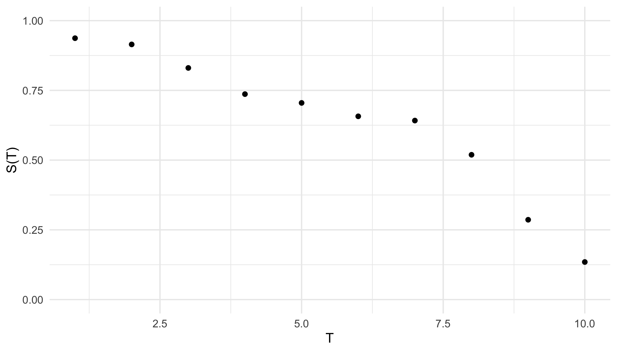
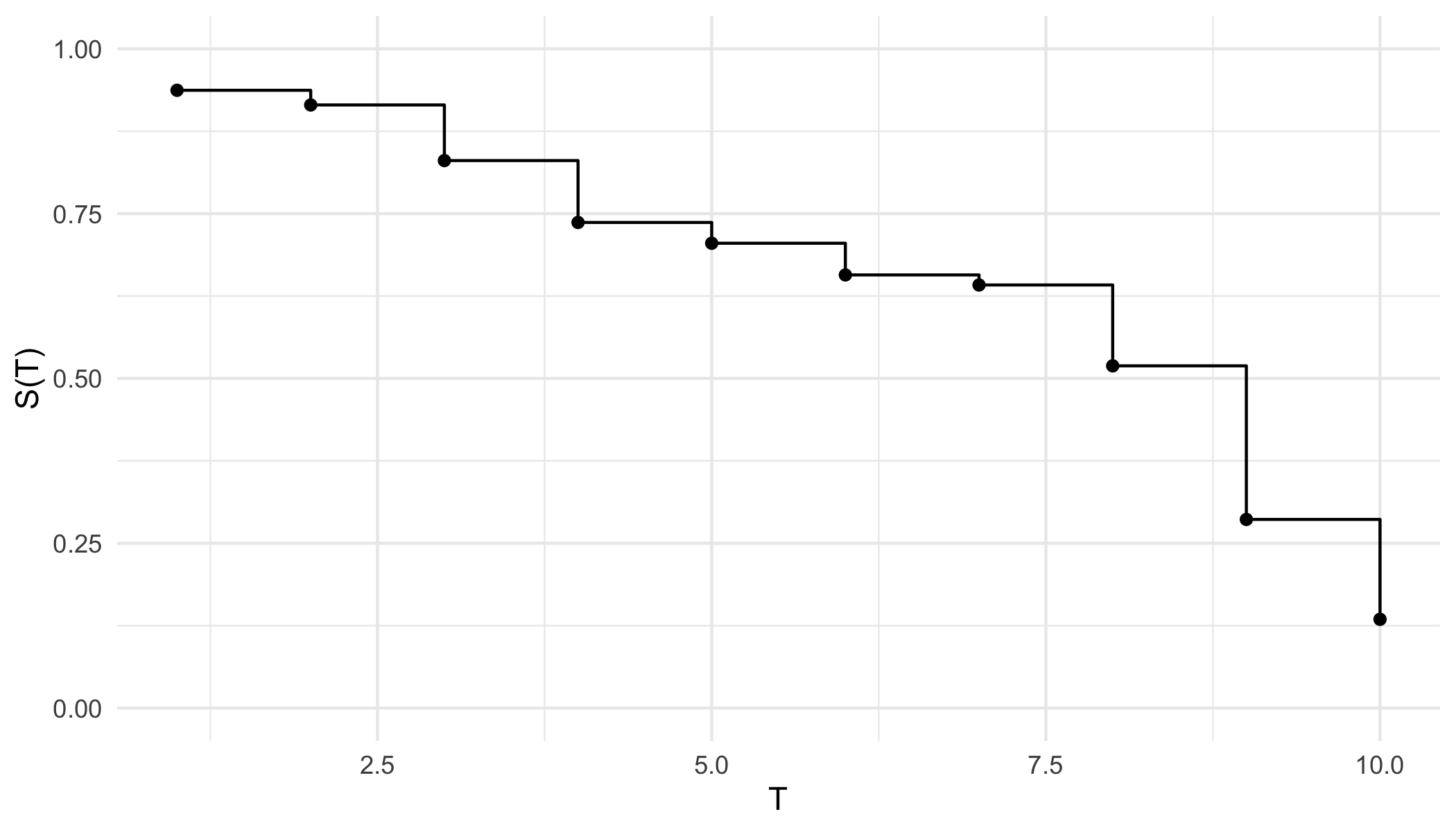
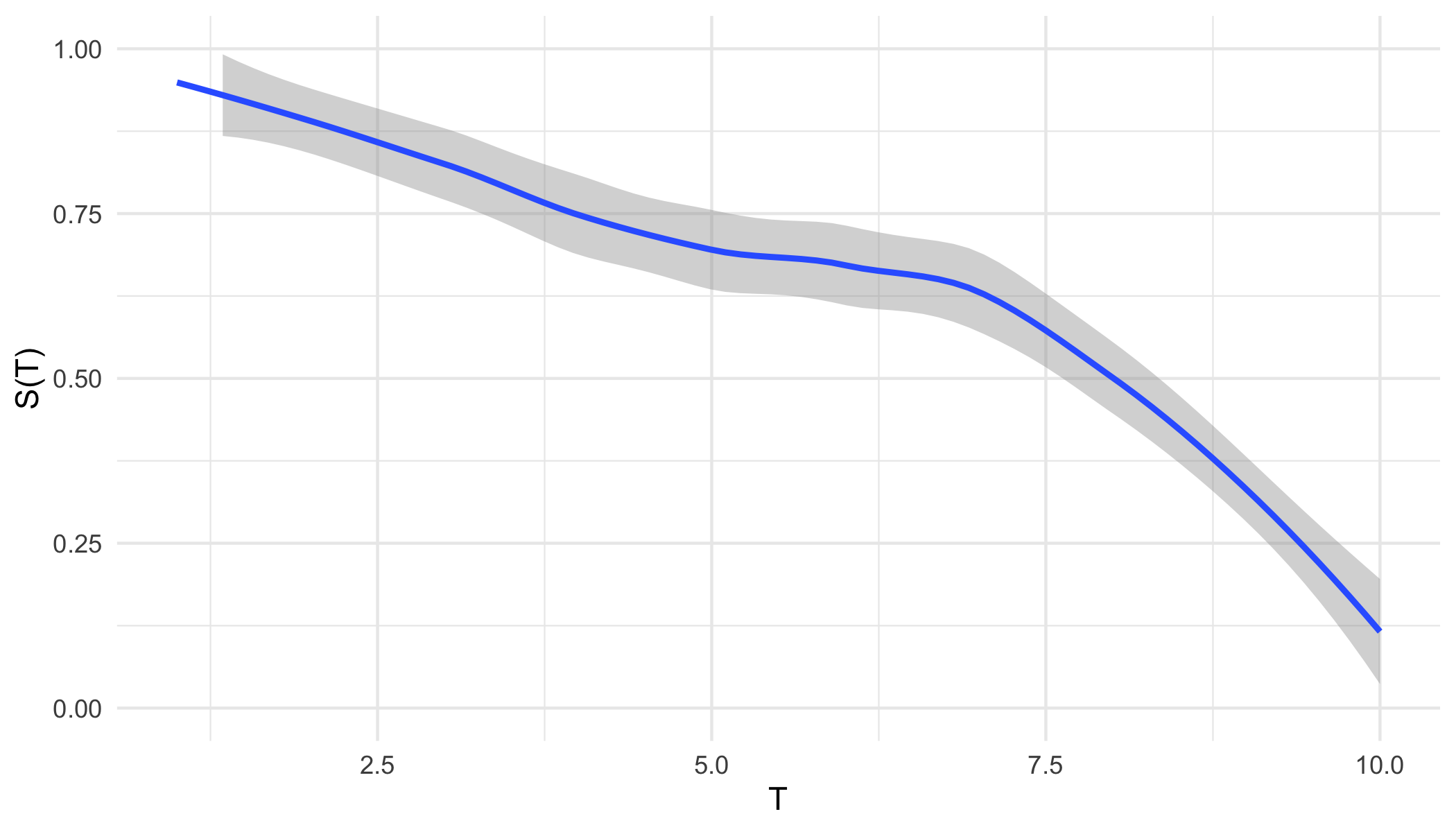
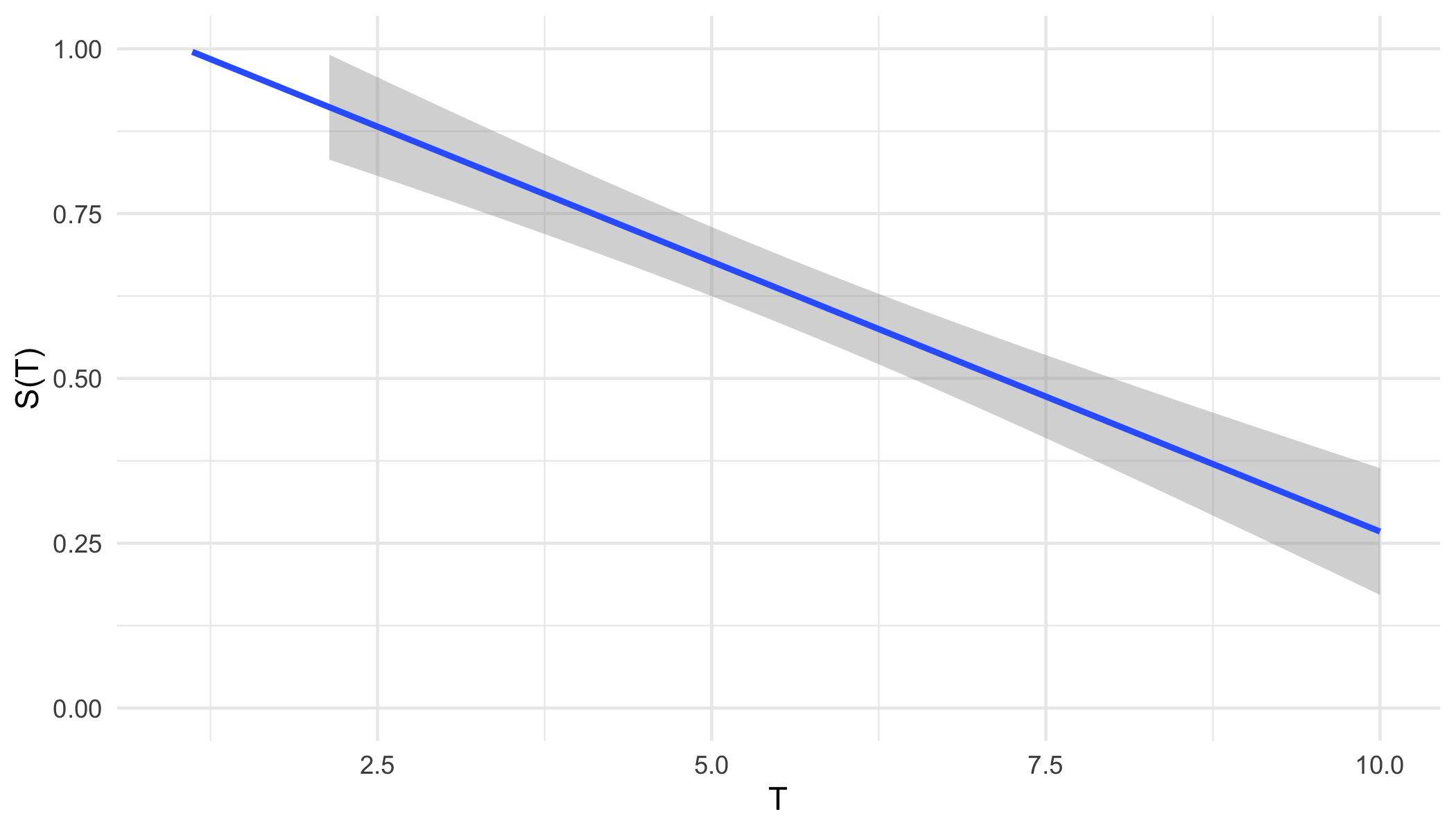
From either representation, a \ non-increasing but non-continuous pseudo-survival function, \(\tilde{S}\), is now predicted. Creating a right-continuous function (‘\(T_1(\tilde{S})\)’ in ?fig-car-R7) from these point predictions (Figure 19.3 (a)) is relatively simple and well-known with accessible off-shelf software. At the very least, one can assume a constant hazard rate between predictions and cast them into a step function (Figure 19.3 (b)). This is a fairly common assumption and is usually valid as bin-width decreases. Alternatively, the point predictions can be smoothed into a continuous function with off-shelf software, for example with polynomial local regression smoothing (Figure 19.3 (c)) or generalised linear smoothing (Figure 19.3 (d)). Whichever method is chosen, the survival function is now non-increasing right-continuous and the (R7) reduction is complete.
ggplot2 (Wickham 2016).
19.5.1.7 R8) Deterministic Survival \(\rightarrow\) Probabilistic Classification
Predicting a deterministic survival time from the multi-label classification predictions is relatively straightforward and can be viewed as a discrete analogue to (C3) (Section 19.4.3). For the discrete hazard representation, one can simply take the predicted time-point for an individual to be time at which the predicted hazard probability is highest however this could easily be problematic as there may be multiple time-points at which the predicted hazard equals \(1\). Instead it is cleaner to first cast the hazard to a pseudo-survival probability (Section 19.5.1.6) and then treat both representations the same.
Let \(\tilde{S}_i\) be the predicted multi-label survival probabilities for an observation \(i\) such that \(\tilde{S}_i(\tau)\) corresponds with \(\hat{P}(Y_{i;\tau} = 1)\) for label \(\tau \in \mathcal{K}\) where \(Y_{i;\tau}\) is defined in Section 19.5.1.2 and \(\mathcal{K} = \{1,...,K\}\) is the set of labels for which to make predictions. Then the survival time transformation is defined by \[ T_2(\tilde{S}_i) = \inf \{\tau \in \mathcal{K} : \tilde{S}_i(\tau) \leq \beta\} \] for some \(\beta \in [0, 1]\).
This is interpreted as defining the predicted survival time as the first time-point in which the predicted probability of being alive drops below a certain threshold \(\beta\). Usually \(\beta = 0.5\), though this can be treated as a hyper-parameter for tuning. This composition can be utilised even if predictions are not non-increasing, as only the first time the predicted survival probability drops below the threshold is considered. With this composition the (R8) reduction is now complete.
19.6 Conclusions
This chapter introduced composition and reduction to survival analysis and formalised specific strategies. Formalising these concepts allows for better quality of research and most importantly improved transparency. Clear interface points for hyper-parameters and compositions allow for reproducibility that was previously obfuscated by unclear workflows and imprecise documentation for pipelines.
Additionally, composition and reduction improves accessibility. Reduction workflows vastly increase the number of machine learning models that can be utilised in survival analysis, thus opening the field to those whose experience is limited to regression or classification. Formalisation of workflows allows for precise implementation of model-agnostic pipelines as computational objects, as opposed to functions that are built directly into an algorithm without external interface points.
Finally, predictive performance is also increased by these methods, which is most prominently the case for the survival model averaging compositor (as demonstrated by RSFs).
All compositions in this chapter, as well as (R1)-(R6), have been implemented in mlr3proba with the mlr3pipelines (Binder et al. 2019) interface. The reductions to classification will be implemented in a near-future update. Additionally the discSurv package (Welchowski and Schmid 2019) will be interfaced as a mlr3proba pipeline to incorporate further discrete-time strategies.
The compositions and are included in the benchmark experiment in R. E. B. Sonabend (2021) so that every tested model can make probabilistic survival distribution predictions as well as deterministic survival time predictions. Future research will benchmark all the pipelines in this chapter and will cover algorithm and model selection, tuning, and comparison of performance. Strategies from other papers will also be explored.