8 Discrimination Measures
This page is a work in progress and minor changes will be made over time.
The next measures discused are ‘discrimination measures’, which evaluate how well models separate observations into different risk groups. A model is said to have good discrimination if it correctly predicts that one observation is at higher risk of the event of interest than another, where the prediction is ‘correct’ if the observation predicted to be at higher risk does indeed experience the event sooner.
In the survival setting, the ‘risk’ is taken to be the continuous ranking prediction. All discrimination measures are ranking measures, which means that the exact predicted value is irrelevant, only its relative ordering is required. For example given predictions \(\{100,2,299.3\}\), only their rankings, \(\{2,1,3\}\), are used by measures of discrimination.
This chapter begins with time-independent measures (Section 8.1), which measure concordance between pairs of observations at a single observed time point. The next section focuses on time-dependent measures (Section 8.2), which are primarily AUC-type measures that evaluate discrimination over all possible unique time-points and integrate the results for a single metric.
8.1 Time-Independent Measures
The simplest form of discrimination measures are concordance indices, which, in general, measure the proportion of cases in which the model correctly ranks a pair of observations according to their risk. These measures may be best understood in terms of two key definitions: ‘comparable’, and ‘concordant’.
Definition 8.1 (Concordance) Let \((i,j)\) be a pair of observations with outcomes \(\{(t_i,\delta_i),(t_j,\delta_j)\}\) and let \(r_i,r_j \in \mathbb{R}\) be their respective risk predictions. Then \((i,j)\) are called (F. E. J. Harrell et al. 1984; F. E. Harrell, Califf, and Pryor 1982):
- Comparable if \(t_i < t_j\) and \(\delta_i = 1\);
- Concordant if \(r_i > r_j\).
Note that this book defines risk rankings such that a higher value implies higher risk of event and thus lower expected survival time (Section 6.1), hence a pair is concordant if \(\mathbb{I}(t_i < t_j, r_i > r_j)\). Other sources may instead assume that higher values imply lower risk of event and hence a pair would be concordant if \(\mathbb{I}(t_i < t_j, r_i < r_j)\).
Concordance measures then estimate the probability of a pair being concordant, given that they are comparable:
\[P(r_i > r_j | t_i < t_j \cap \delta_i)\]
These measures are referred to as time independent when \(r_i,r_j\) is not a function of time as once the observations are organised into comparable pairs, the observed survival times can be ignored. The time-dependent case is covered in Section 8.2.1.
While various definitions of a ‘Concordance index’ (C-index) exist (discussed in the next section), they all represent a weighted proportion of the number of concordant pairs over the number of comparable pairs. As such, a C-index value will always be between \([0, 1]\) with \(1\) indicating perfect separation, \(0.5\) indicating no separation, and \(0\) being separation in the ‘wrong direction’, i.e. all high risk observations being ranked lower than all low risk observations.
Concordance measures may either be reported as a value in \([0,1]\), a percentage, or as ‘discriminatory power’, which refers to the percentage improvement of a model’s discrimination above the baseline value of \(0.5\). For example, if a model has a concordance of \(0.8\) then its discriminatory power is \((0.8-0.5)/0.5 = 60\%\). This representation of discrimination provides more information by encoding the model’s improvement over some baseline although is often confused with reporting concordance as a percentage (e.g. reporting a concordance of 0.8 as 80%). In theory this representation could result in a negative value, however this would indicate that \(C<0.5\), which would indicate serious problems with the model that should be addressed before proceeding with further analysis. Representing measures as a percentage over a baseline is a common method to improve measure interpretability and closely relates to the ERV representation of scoring rules.
8.1.1 Concordance Indices
Common concordance indices in survival analysis can be expressed as a general measure:
Let \(\boldsymbol{\hat{r}} = ({\hat{r}}_1 \ {\hat{r}}_2 \cdots {\hat{r}}_{m})^\intercal\) be predicted risks, \((\mathbf{t}, \boldsymbol{\delta}) = ((t_1, \delta_1) \ (t_2, \delta_2) \cdots (t_m, \delta_m))^\intercal\) be observed outcomes, let \(W\) be some weighting function, and let \(\tau\) be a cut-off time. Then, the time-independent (‘ind’) survival concordance index is defined by,
\[ C_{ind}(\hat{\mathbf{r}}, \mathbf{t}, \boldsymbol{\delta}|\tau) = \frac{\sum_{i\neq j} W(t_i)\mathbb{I}(t_i < t_j, \hat{r}_i > \hat{r}_j, t_i < \tau)\delta_i}{\sum_{i\neq j}W(t_i)\mathbb{I}(t_i < t_j, t_i < \tau)\delta_i} \]
The choice of \(W\) specifies a particular variation of the c-index (see below). The use of the cut-off \(\tau\) mitigates against decreased sample size (and therefore high variance) over time due to the removal of censored observations (see Figure 8.1)). For \(\tau\) to be comparable across datasets, a common choice would be to set \(\tau\) as the time at which 80%, or perhaps 90% of the data have been censored or experienced the event.
There are multiple methods for dealing with tied predictions and times. Strictly, tied times are incomparable given the definition of ‘comparable’ given above and hence are usually ignored in the numerator. On the other hand, ties in the prediction are more problematic but a common method is to set a value of \(0.5\) for observations when \(r_i = r_j\) (Therneau and Atkinson 2020). Specific concordance indices can be constructed by assigning a weighting scheme for \(W\) which generally depends on the Kaplan-Meier estimate of the survival function of the censoring distribution fit on training data, \(\hat{G}_{KM}\), or the Kaplan-Meier estimate for the survival function of the survival distribution fit on training data, \(\hat{S}_{KM}\), or both. Measures that use \(\hat{G}_{KM}\) are referred to as Inverse Probability of Censoring Weighted (IPCW) measures as the estimated censoring distribution is utilised to weight the measure in order to compensate for removed censored observations. This is visualised in Figure 8.1 where \(\hat{G}_{KM}\), \(\hat{G}_{KM}^{-2}\), and \(\hat{S}_{KM}\) are computed based on the whas dataset (Hosmer Jr, Lemeshow, and May 2011).
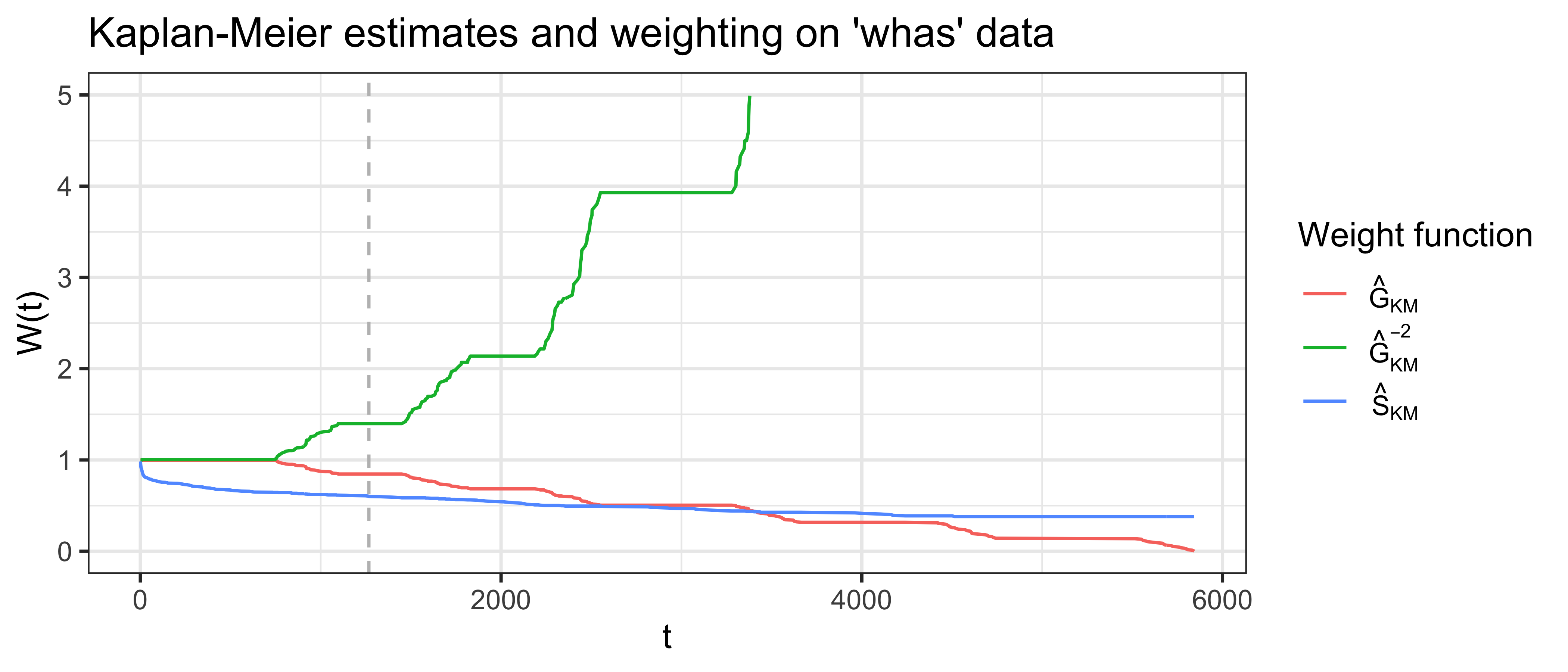
whas dataset. x-axis is follow-up time. y-axis is outputs from one of three weighting functions: \(\hat{G}_{KM}\), survival function based on the censoring distribution of the whas dataset (red), and \(\hat{G}_{KM}^{-2}\) (green), \(\hat{S}_{KM}\), marginal survival function based on original whas dataset (blue), . The vertical gray line at \(t = \tau=1267\) represents the point at which \(\hat{G}(t)<0.6\).
The following weights have been proposed for the concordance index:
- \(W(t_i) = 1\): Harrell’s concordance index, \(C_H\) (F. E. J. Harrell et al. 1984; F. E. Harrell, Califf, and Pryor 1982), which is widely accepted to be the most common survival measure and imposes no weighting on the definition of concordance. The original measure given by Harrell has no cut-off, \(\tau = \infty\), however applying a cut-off is now more widely accepted in practice.
- \(W(t_i) = [\hat{G}_{KM}(t_i)]^{-2}\): Uno’s C, \(C_U\) (Uno et al. 2011).
- \(W(t_i) = [\hat{G}_{KM}(t_i)]^{-1}\)
- \(W(t_i) = \hat{S}_{KM}(t_i)\)
- \(W(t_i) = \hat{S}_{KM}(t_i)/\hat{G}_{KM}(t_i)\)
All methods assume that censoring is conditionally-independent of the event given the features (?sec-surv-set-cens), otherwise weighting by \(\hat{S}_{KM}\) or \(\hat{G}_{KM}\) would not be applicable. It is assumed here that \(\hat{S}_{KM}\) and \(\hat{G}_{KM}\) are estimated on the training data and not the testing data (though the latter may be seen in some implementations, e.g. Therneau (2015)).
8.1.2 Choosing a C-index
With multiple choices of weighting available, choosing a specific measure might seem daunting. Matters are only made worse by debate in the literature, reflecting uncertainty in measure choice and interpretation. In practice, when a suitable cut-of \(\tau\) is chosen, all these weightings perform very similarly (Rahman et al. 2017; Schmid and Potapov 2012). For example, Table 8.1 uses the whas data again to compare Harrell’s C with measures that include IPCW weighting, when no cutoff is applied (top row) and when a cutoff is applied when \(\hat{G}(t)=0.6\) (grey line in Figure 8.1). The results are almost identical when the cutoff is applied but still not massively different without the cutoff.
whas dataset using a Cox model with three-fold cross-validation) with no cut-off (top) and a cut-off when \(\hat{G}(t)=0.6\) (bottom). First column is Harrell’s C, second is the weighting \(1/\hat{G}(t)\), third is Uno’s C.
| \(W=1\) | \(W= G^{-1}\) | \(W=G^{-2}\) | |
|---|---|---|---|
| \(\tau=\infty\) | 0.74 | 0.73 | 0.71 |
| \(\tau=1267\) | 0.76 | 0.75 | 0.75 |
On the other hand, if a poor choice is selected for \(\tau\) (cutting off too late) then IPCW measures can be highly unstable (Rahman et al. 2017), for example the variance of Uno’s C drastically increases with increased censoring (Schmid and Potapov 2012).
In practice, all C-index metrics provide an intuitive measure of discrimination and as such the choice of C-index is less important than the transparency in reporting. ‘C-hacking’ (R. Sonabend, Bender, and Vollmer 2022) is the deliberate, unethical procedure of calculating multiple C-indices and to selectively report one or more results to promote a particular model or result, whilst ignoring any negative findings. For example, calculating Harrell’s C and Uno’s C but only reporting the measure that shows a particular model of interest is better than another (even if the other metric shows the reverse effect). To avoid ‘C-hacking’:
- the choice of C-index should be made before experiments have begun and the choice of C-index should be clearly reported;
- when ranking predictions are composed from distribution predictions, the composition method should be chosen and clearly described before experiments have begun.
As the C-index is highly dependent on censoring within a dataset, C-index values between experiments are not directly comparable, instead comparisons are limited to comparing model rankings, for example conclusions such as “model A outperformed model B with respect to Harrell’s C in this experiment”.
8.2 Time-Dependent Measures
In the time-dependent case, where the metrics are computed based on specific survival times, the majority of measures are based on the Area Under the Curve, with one exception which is a simpler concordance index.
8.2.1 Concordance Indices
In contrast to the measures described above, Antolini’s C (Antolini, Boracchi, and Biganzoli 2005) provides a time-dependent (‘dep’) formula for the concordance index. The definition of ‘comparable’ is the same for Antolini’s C, however, concordance is now determined using the individual predicted survival probabilities calculated at the smaller event time in the pair:
\[P(\hat{S}_i(t_i) < \hat{S}_j(t_i) | t_i < t_j \cap \delta_i)\]
Note that observations are concordant when \(\hat{S}_i(t_i) < \hat{S}_j(t_i)\) as at the time \(t_i\), observation \(i\) has experienced the event and observation \(j\) has not, hence the expected survival probability for \(\hat{S}_i(t_i)\) should be as close to 0 as possible (noting inherent randomness may prevent the perfect \(\hat{S}_i(t_i)=0\) prediction) but otherwise should be less than \(\hat{S}_j(t_i)\) as \(j\) is still ‘alive’. Once again this probability is estimated with a metric that could include a cut-off and different weighting schemes (though this is not included in Antolini’s original definition):
\[ C_{dep}(\hat{\mathbf{S}}, \mathbf{t}, \boldsymbol{\delta}|\tau) = \frac{\sum_{i\neq j} W(t_i)\mathbb{I}(t_i < t_j, \hat{S}_i(t_i) < \hat{S}_j(t_i), t_i < \tau)\delta_i}{\sum_{i\neq j}W(t_i)\mathbb{I}(t_i < t_j, t_i < \tau)\delta_i} \]
where \(\boldsymbol{\hat{S}} = ({\hat{S}}_1 \ {\hat{S}}_2 \cdots {\hat{S}}_{m})^\intercal\).
Antolini’s C provides an intuitive method to evaluate the discrimination of a model based on distribution predictions without depending on compositions to ranking predictions.
8.2.2 Area Under the Curve
We are still discussing how to structure and write this section so the contents are all subject to change. The text below is ‘correct’ but we want to add more detail about estimation of AUC so the book can be more practical, otherwise we may remove the section completely, let us know your thoughts about what you’d like to see here!
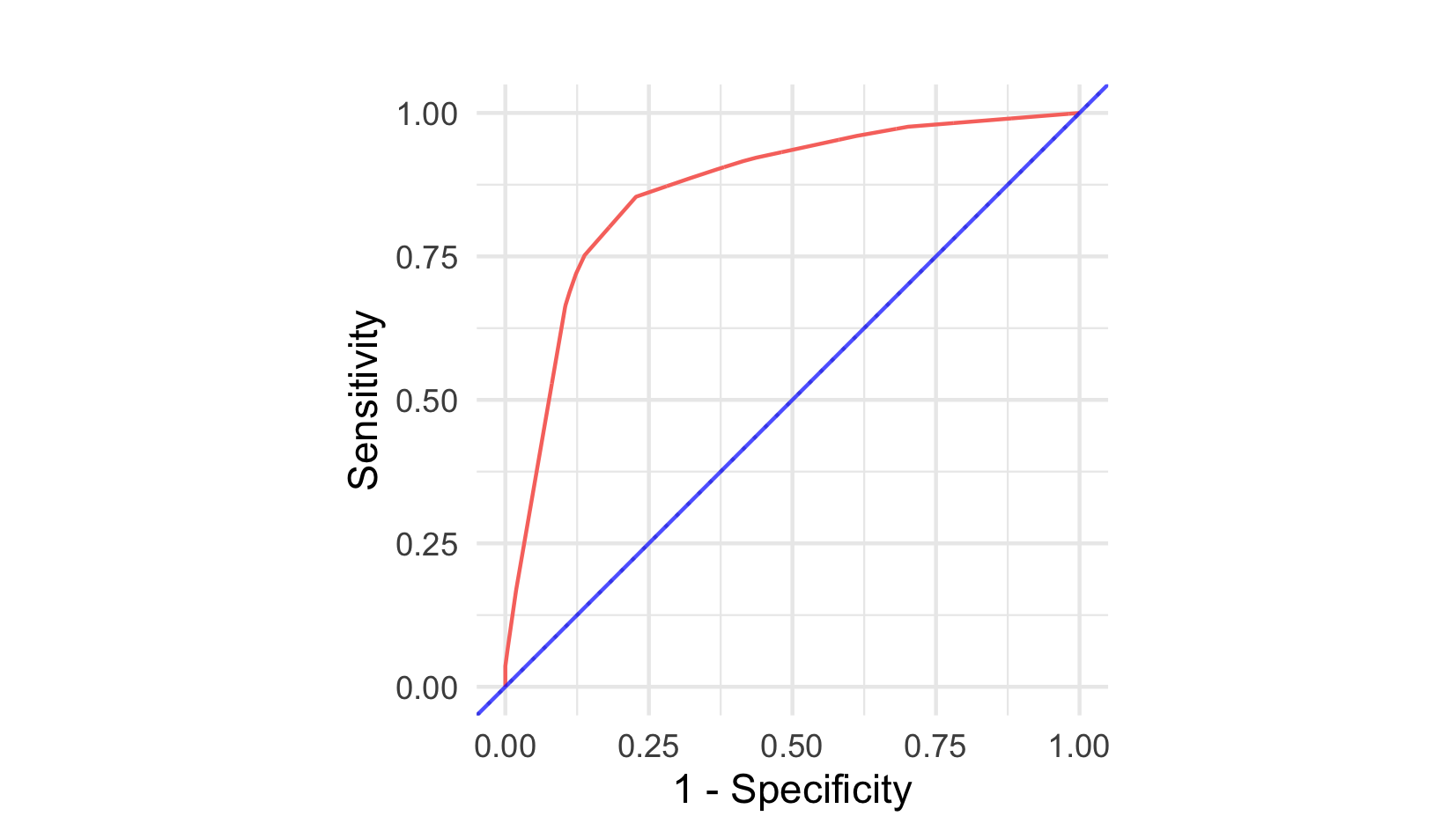
AUC, or AUROC, measures calculate the Area Under the Receiver Operating Characteristic (ROC) Curve, which is a plot of the sensitivity (or true positive rate (TPR)) against \(1 - \textit{specificity}\) (or true negative rate (TNR)) at varying thresholds (described below) for the predicted probability (or risk) of event. Figure 8.2 visualises ROC curves for two classification models. The blue line is a featureless baseline that has no discrimination. The red line is a decision tree with better discrimination as it comes closer to the top-left corner.
In a classification setting with no censoring, the AUC has the same interpretation as Harrell’s C (Uno et al. 2011). AUC measures for survival analysis were developed to provide a time-dependent measure of discriminatory ability (Patrick J. Heagerty, Lumley, and Pepe 2000). In a survival setting it can reasonably be expected for a model to perform differently over time and therefore time-dependent measures are advantageous. Computation of AUC estimators is complex and as such there are limited accessible metrics available off-shelf. There is limited evidence of these estimators used in the literature, hence discussion of these measures is kept brief.
The AUC, TPR, and TNR are derived from the confusion matrix in a binary classification setting. Let \(b_i,\hat{b}_i \in \{0, 1\}\) be the true and predicted binary outcomes respectively for some observation \(i\). The confusion matrix is then given by:
| \(b_i = 1\) | \(b_i = 0\) | |
| \(\hat{b}_i = 1\) | TP | FP |
| \(\hat{b}_i = 0\) | FN | TN |
where \(TN := \sum_i \mathbb{I}(b_i = 0, \hat{b}_i = 0)\) is the number of true negatives, \(TP := \sum_i \mathbb{I}(b_i = 1, \hat{b}_i = 1)\) is the number true positives, \(FP := \sum_i \mathbb{I}(b_i = 0, \hat{b}_i = 1)\) is the number of false positives, and \(FN := \sum_i \mathbb{I}(b_i = 1, \hat{b}_i = 0)\) is the number of false negatives. From these are derived
\[\begin{align} & TPR := \frac{TP}{TP + FN} \\ & TNR := \frac{TN}{TN + FP} \end{align}\]
In classification, a probabilistic prediction of an event can be thresholded to obtain a deterministic prediction. For a predicted \(\hat{p} := \hat{P}(b = 1)\), and threshold \(\alpha\), the thresholded binary prediction is \(\hat{b} := \mathbb{I}(\hat{p} > \alpha)\). This is achieved in survival analysis by thresholding the linear predictor at a given time for different values of the threshold and different values of the time. All measures of TPR, TNR and AUC are in the range \([0,1]\) with larger values preferred.
Weighting the linear predictor was proposed by Uno \(\textit{et al.}\) (2007) (Uno et al. 2007) and provides a method for estimating TPR and TNR via
\[ \begin{split} &TPR_U(\boldsymbol{\hat{\eta}}, \mathbf{t}, \boldsymbol{\delta}| \tau, \alpha) = \frac{\sum^m_{i=1} \delta_i \mathbb{I}(k(\hat{\eta}_i) > \alpha, t_i \leq \tau)[\hat{G}_{KM}(t_i)]^{-1}}{\sum^m_{i=1}\delta_i\mathbb{I}(t_i \leq \tau)[\hat{G}_{KM}(t_i)]^{-1}} \end{split} \]
and
\[ \begin{split} &TNR_U(\boldsymbol{\hat{\eta}}, \mathbf{t}| \tau, \alpha) \mapsto \frac{\sum^m_{i=1} \mathbb{I}(k(\hat{\eta}_i) \leq \alpha, t_i > \tau)}{\sum^m_{i=1}\mathbb{I}(t_i > \tau)} \end{split} \] where \(\boldsymbol{\hat{\eta}} = ({\hat{\eta}}_1 \ {\hat{\eta}}_2 \cdots {\hat{\eta}}_{m})^\intercal\) is a vector of predicted linear predictors, \(\tau\) is the time at which to evaluate the measure, \(\alpha\) is a cut-off for the linear predictor, and \(k\) is a known, strictly increasing, differentiable function. \(k\) is chosen depending on the model choice, for example if the fitted model is PH then \(k(x) = 1 - \exp(-\exp(x))\) (Uno et al. 2007). Similarities can be drawn between these equations and Uno’s concordance index, in particular the use of IPCW. Censoring is again assumed to be at least random once conditioned on features. Plotting \(TPR_U\) against \(1 - TNR_U\) for varying values of \(\alpha\) provides the ROC.
The second method, which appears to be more prominent in the literature, is derived from Heagerty and Zheng (2005) (Patrick J. Heagerty and Zheng 2005). They define four distinct classes, in which observations are split into controls and cases.
An observation is a case at a given time-point if they are dead, otherwise they are a control. These definitions imply that all observations begin as controls and (hypothetically) become cases over time. Cases are then split into incident or cumulative and controls are split into static or dynamic. The choice between modelling static or dynamic controls is dependent on the question of interest. Modelling static controls implies that a ‘subject does not change disease status’ (Patrick J. Heagerty and Zheng 2005), and few methods have been developed for this setting (Kamarudin, Cox, and Kolamunnage-Dona 2017), as such the focus here is on dynamic controls. The incident/cumulative cases choice is discussed in more detail below.1
1 All measures discussed in this section evaluate model discrimination from ‘markers’, which may be a predictive marker (model predictions) or a prognostic marker (a single covariate). This section always defines a marker as a ranking prediction, which is valid for all measures discussed here with the exception of one given at the end.
The TNR for dynamic cases is defined as
\[ TNR_D(\hat{\mathbf{r}}, N | \alpha, \tau) = P(\hat{r}_i \leq \alpha | N_i(\tau) = 0) \] where \(\boldsymbol{\hat{r}} = ({\hat{r}}_1 \ {\hat{r}}_2 \cdots {\hat{r}}_{n})^\intercal\) is some deterministic prediction and \(N(\tau)\) is a count of the number of events in \([0,\tau)\). Heagerty and Zheng further specify \(y\) to be the predicted linear predictor \(\hat{\eta}\). Cumulative/dynamic and incident/dynamic measures are available in software packages ‘off-shelf’, these are respectively defined by
\[ TPR_C(\hat{\mathbf{r}}, N | \alpha, \tau) = P(\hat{r}_i > \alpha | N_i(\tau) = 1) \] and
\[ TPR_I(\hat{\mathbf{r}}, N | \alpha, \tau) = P(\hat{r}_i > \alpha | dN_i(\tau) = 1) \] where \(dN_i(\tau) = N_i(\tau) - N_i(\tau-)\). Practical estimation of these quantities is not discussed here.
The choice between the incident/dynamic (I/D) and cumulative/dynamic (C/D) measures primarily relates to the use-case. The C/D measures are preferred if a specific time-point is of interest (Patrick J. Heagerty and Zheng 2005) and is implemented in several applications for this purpose (Kamarudin, Cox, and Kolamunnage-Dona 2017). The I/D measures are preferred when the true survival time is known and discrimination is desired at the given event time (Patrick J. Heagerty and Zheng 2005).
Defining a time-specific AUC is now possible with
\[ AUC(\hat{\mathbf{r}}, N | \tau) = \int^1_0 TPR(\hat{\mathbf{r}}, N | 1 - TNR^{-1}(p|\tau), \tau) \ dp \]
Finally, integrating over all time-points produces a time-dependent AUC and as usual a cut-off is applied for the upper limit,
\[ AUC^*(\hat{\mathbf{r}},N|\tau^*) = \int^{\tau^*}_0 AUC(\hat{\mathbf{r}},N|\tau)\frac{2\hat{p}_{KM}(\tau)\hat{S}_{KM}(\tau)}{1 - \hat{S}_{KM}^2(\tau^*)} \ d\tau \] where \(\hat{S}_{KM},\hat{p}_{KM}\) are survival and mass functions estimated with a Kaplan-Meier model on training data.
Since Heagerty and Zheng’s paper, other methods for calculating the time-dependent AUC have been devised, including by Chambless and Diao (Chambless and Diao 2006), Song and Zhou (Song and Zhou 2008), and Hung and Chiang (Hung and Chiang 2010). These either stem from the Heagerty and Zheng paper or ignore the case/control distinction and derive the AUC via different estimation methods of TPR and TNR. Blanche \(\textit{et al.}\) (2012) (Blanche, Latouche, and Viallon 2012) surveyed these and concluded ‘’regarding the choice of the retained definition for cases and controls, no clear guidance has really emerged in the literature’‘, but agree with Heagerty and Zeng on the use of C/D for clinical trials and I/D for ’pure’ evaluation of the marker. Blanche \(\textit{et al.}\) (2013) (Blanche, Dartigues, and Jacqmin-Gadda 2013) published a survey of C/D AUC measures with an emphasis on non-parametric estimators with marker-dependent censoring, including their own Conditional IPCW (CIPCW) AUC, which is not discussed further here as it cannot be used for evaluating predictions (R. E. B. Sonabend 2021).
Reviews of AUC measures have produced (sometimes markedly) different results (Blanche, Latouche, and Viallon 2012; Li, Greene, and Hu 2018; Kamarudin, Cox, and Kolamunnage-Dona 2017) with no clear consensus on how and when these measures should be used. The primary advantage of these measures is to extend discrimination metrics to be time-dependent. However, it is unclear how to interpret a threshold of a linear predictor and moreover if this is even the ‘correct’ quantity to threshold, especially when survival distribution predictions are the more natural object to evaluate over time.