5 Event-history Analysis
This page is a work in progress and major changes will be made over time.
In this section we will go beyond single-event data or at least view time-to-event data more generally as data in which one could observe multiple, potentially mutually exclusive events. From this more general point of view such data is sometimes refered to event-history data and its analysis as event-history analysis (EHA). The table below gives one way to classify the different types of data that could occur in EHA, where we differentiate between the number of occurences of the same event type (rows) and whether we consider the occurence of the same event or different events (columns).
| single outcome | many outcomes | |
|---|---|---|
| one/first event | single event | competing risks |
| multiple events | recurrent events | multi state |
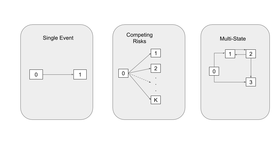
Another way to think about event history is in terms of transitions between different states, as illustrated in Figure 5.1. Usually, a subject starts out in state 0 (for example, healthy) and transitions to different states from there. States from which further transitions are possible are called transient, otherwise a state is called terminal. If no transition happens within the follow-up time, the subject remains in the initial state, in event history terms the observation is censored for this transition.
In the single-event setting (Figure 5.1, left panel), a subject can only transition to one state (the event of interest). In the competing risks setting (Figure 5.1, middle panel, see Section 5.1), a subject could transition to any of the \(K\) mutually exclusive states, thus the subject is at risk for a transition to multiple states. However, once one of them occurs, it is impossible to transition to another (for example, death from different causes). In both cases, the event needs not be terminal, we just end the observation after the first occurence of an event.
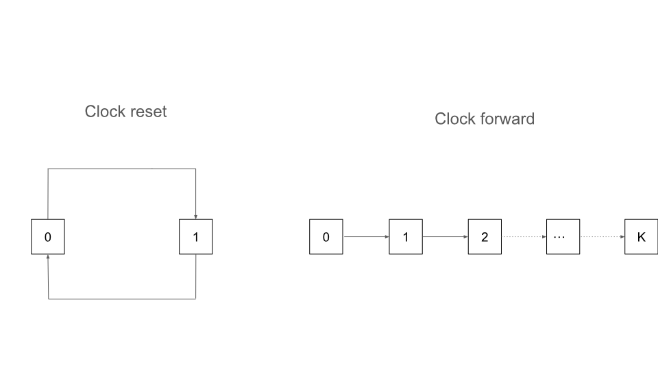
In the most general case, the multi-state setting (Figure 5.1 right panel, see Section 5.2), there are multiple transient and terminal states with potential back transitions (for example, moving between different stages of an illness with the possibility of (partial) recovery and death as terminal event). The recurrent events setting is as a special case of the multi-state setting but could also be treated as a more general case of the single event setting with correlated observations (Section 5.3 and Figure 5.2) .
5.1 Competing Risks
In constrast to single-event survival analysis, competing risks are concerned with the time to the first of many, mutually exclusive events. Mutually exclusive here means that once one of the events occurs, we can not observe the others. As in the single event case, the events may not necessarily be terminal (such as death), instead they just signify the end of the period of interest for a given observation.
Formally, let \(Y\) be the time-to-event as before. In the competing risks setting, there is now an additional random variable \(E_Y\in \{1,\ldots,k\}\), which denotes one of \(k\) competing events that can occur at event time \(Y\). The survival outcome notation, \((T, \Delta)\) has to be extended to accomodate for the possible competing risks. Previously, \(\Delta = 1\) if right-censoring is observed, this can be modified by multiplying \(\Delta\) by the index of the event that occurs. Now, \(\Delta \in \{0, 1, \ldots, k\}\) where \(\Delta = 0\) still indicates censoring and \(\Delta = j\) means the \(j\)th event occurred.
The predominate approach to competing-risks analysis is known as cause-specific hazards, where \(h_{0e}\) is defined as the hazard for the transition from initial state \(0\) to state \(e =1,\ldots,k\):
\[ h_{0e}(\tau) = \lim_{\Delta \tau \to 0} \frac{P(\tau \leq Y \leq \tau + \Delta \tau, E = e\ |\ Y \geq \tau)}{\Delta \tau}, \; e = 1, \dots, k. \]
As competing events are mutually exclusive at any time \(\tau\), it is useful to further define the:
- all-cause hazard, \(h(\tau) = \sum_{e = 1}^{k}h_{0e}(\tau)\): which is the…
- all-cause cumulative hazard: \(H(\tau) = \int_{0}^\tau h(u)\ du = \sum_{e=1}^{k}\int_{0}^\tau h_{0e}(u)\ du = \sum_{e=1}^k H_{0e}(\tau)\), and
- all-cause survival probability: \(S(\tau) = P(Y \geq \tau) = \exp(-H(\tau))\)
Note that whilst the all-cause survival probability is defined in the same way as the standard survival probability, the interpretation is that none of the events occurred before \(\tau\). The all-cause survival probability is also not directly estimated but instead calculated from the cause specific hazards.
Another important distribution function in competing risks analysis is the Cumulative Incidence Function (CIF), which denotes the probability of experiencing an event \(E\) before time \(\tau\)
\[ F_{e}(\tau) = P(Y \leq \tau, E = e) = \int_{0}^\tau h_{0e}(u)S(u)\ du. \] Intuitively the CIF is the probability of not experiencing any event, \(S(u)\), multiplied with the hazard of experiencing an event of type \(e\), \(h_{oe}(u)\).
Calculating the CIF (in addition to the cause-specific hazards) is particularly important when making statements about the absolute risk (probability) for an event of type \(e\), as it depends on all cause-specific hazards via \(S(\tau)\).
This will be particularly relevant when assesing how features affect the probability for observing a specific event. While some features might strongly affect some of the cause-specific hazards, if an event has overall low prevalence, then the absolute probability of observing the event will still be low. Hence the CIF is useful for incorporating this information into an interpretable quantity.
Following Beyersmann, Allignol, and Schumacher (2012), this book assumes that the cause-specific hazards model fully describes the data generating processes and doesn’t require an independence assumption for the competing events.
5.2 Multi-state Models
This page is a work in progress and major changes will be made over time.
5.3 Recurrent Events
This page is a work in progress and major changes will be made over time.