10 Evaluating Distributions by Scoring Rules
This page is a work in progress and minor changes will be made over time.
Scoring rules evaluate probabilistic predictions and (attempt to) measure the overall predictive ability of a model in terms of both calibration and discrimination (Gneiting and Raftery 2007; Murphy 1973). In contrast to calibration measures, which assess the average performance across all observations on a population level, scoring rules evaluate the sample mean of individual predictions across all observations in a test set. As well as being able to provide information at an individual level, scoring rules are also popular as probabilistic forecasts are widely recognised to be superior to deterministic predictions for capturing uncertainty in predictions (A. P. Dawid 1984; A. Philip Dawid 1986). Formalisation and development of scoring rules has primarily been due to Dawid (A. P. Dawid 1984; A. Philip Dawid 1986; A. Philip Dawid and Musio 2014) and Gneiting and Raftery (Gneiting and Raftery 2007); though the earliest measures promoting “rational” and “honest” decision making date back to the 1950s (Brier 1950; Good 1952). Few scoring rules have been proposed in survival analysis, although the past few years have seen an increase in popularity in these measures. Before delving into these measures, we will first describe scoring rules in the simpler classification setting.
Scoring rules are pointwise losses, which means a loss is calculated for all observations and the sample mean is taken as the final score. To simplify notation, we only discuss scoring rules in the context of a single observation where \(L_i(\hat{S}_i, t_i, \delta_i)\) would be the loss calculated for some observation \(i\) where \(\hat{S}_i\) is the predicted survival function (from which other distribution functions can be derived), and \((t_i, \delta_i)\) is the observed survival outcome.
10.1 Classification Losses
In the simplest terms, a scoring rule compares two values and assigns them a score (hence ‘scoring rule’), formally we’d write \(L: \mathbb{R}\times \mathbb{R}\mapsto \bar{\mathbb{R}}\). In machine learning, this usually means comparing a prediction for an observation to the ground truth, so \(L: \mathbb{R}\times \mathcal{P}\mapsto \bar{\mathbb{R}}\) where \(\mathcal{P}\) is a set of distributions. Crucially, scoring rules usually refer to comparisons of true and predicted distributions. As an example, take the Brier score (Brier 1950) defined by: \[L_{Brier}(\hat{p}_i, y_i) = (y_i - \hat{p}_i(y_i))^2\]
This scoring rule compares the ground truth to the predicted probability distribution by testing if the difference between the observed event and the truth is minimized. This is intuitive as if the event occurs and \(y_i = 1\), then \(\hat{p}_i(y_i)\) should be as close to one as possible to minimize the loss. On the other hand, if \(y_i = 0\) then the better prediction would be \(\hat{p}_i(y_i) = 0\).
This demonstrates an important property of the scoring rule, properness. A loss is proper, if it is minimized by the correct prediction. In contrast, the loss \(L_{improper}(\hat{p}_i, y_i) = 1 - L_{Brier}(\hat{p}_i, y_i)\) is still a scoring rule as it compares the ground truth to the prediction probability distribution, but it is clearly improper as the perfect prediction (\(\hat{p}_i(y_i) = y_i\)) would result in a score of \(1\) whereas the worst prediction would result in a score or \(0\). Proper losses provide a method of model comparison as, by definition, predictions closest to the true distribution will result in lower expected losses.
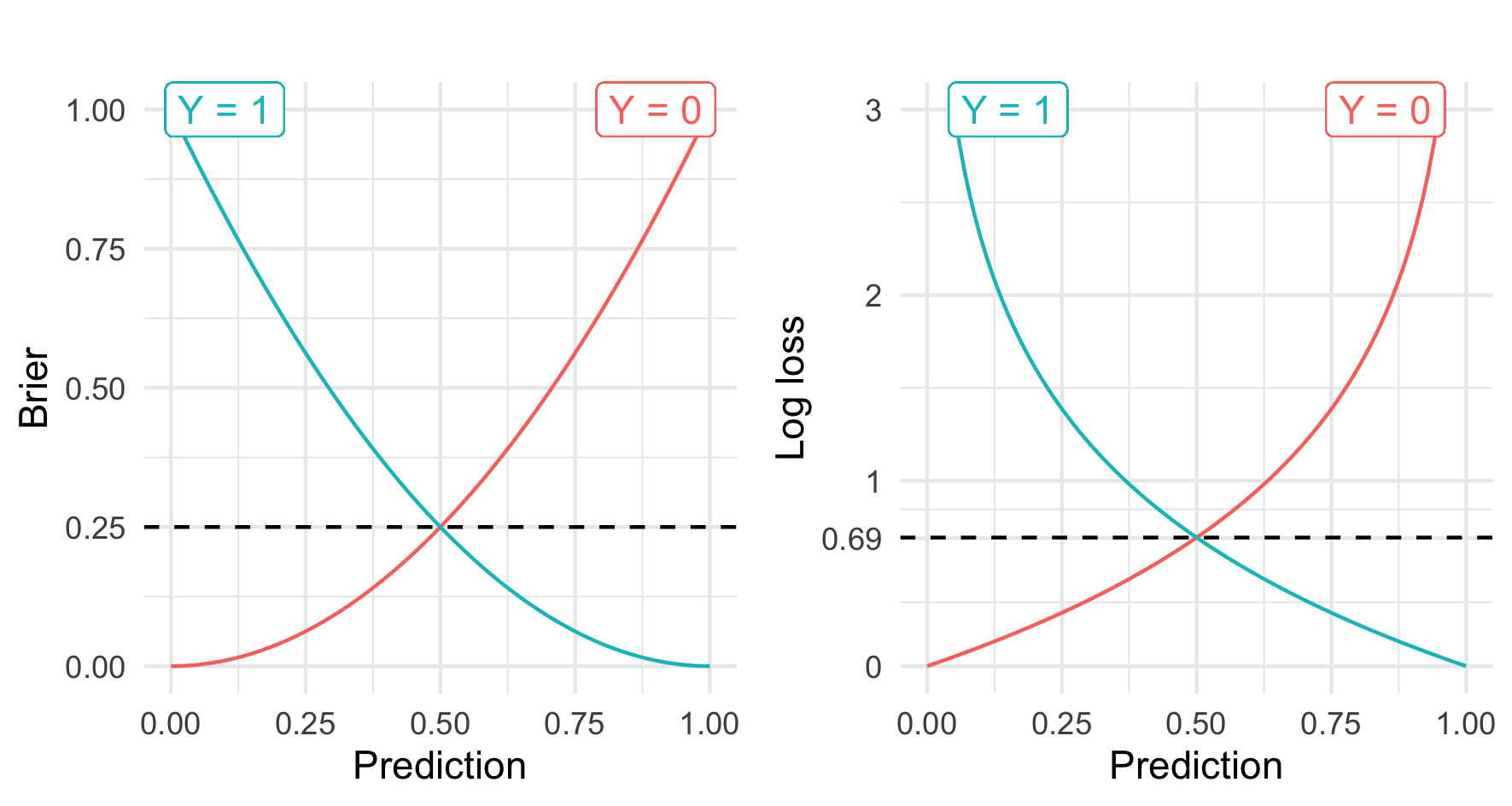
Another important property is strict properness. A loss is strictly proper if the loss is uniquely minimized by the ‘correct’ prediction. Consider now the loss \(L_0(\hat{p}_i, y_i) = 0\). Not only is this a strictly proper scoring rule but it is also proper. The loss can only take the value \(0\) and is therefore guaranteed to be minimized by the correct prediction. It is clear however that this loss is useless. In contrast, the Brier score is minimized by only one value, which is the optimal prediction (Figure 10.1). Strictly proper losses are particular important for automated model optimisation, as minimization of the loss will result in the ‘optimum score estimator based on the scoring rule’ (Gneiting and Raftery 2007).
Mathematically, a classification loss \(L: \mathcal{P}\times \mathcal{Y}\rightarrow \bar{\mathbb{R}}\) is proper if for any distributions \(p_Y,p\) in \(\mathcal{P}\) and for any random variables \(Y \sim p_Y\), it holds that \(\mathbb{E}[L(p_Y, Y)] \leq \mathbb{E}[L(p, Y)]\). The loss is strictly proper if, in addition, \(p = p_Y\) uniquely minimizes the loss.
As well as the Brier score, which was defined above, another widely used loss is the log loss (Good 1952), defined by
\[ L_{logloss}(\hat{p}_i, y_i) = -\log \hat{p}_i(y_i) \]
These losses are visualised in Figure 10.1, which highlights that both losses are strictly proper (A. Philip Dawid and Musio 2014) as they are minimized when the true prediction is made, and converge to the minimum as predictions are increasingly improved.
10.2 Survival Losses
Analogously to classification losses, a survival loss \(L: \mathcal{P}\times \mathbb{R}_{>0}\times \{0,1\}\rightarrow \bar{\mathbb{R}}\) is proper if for any distributions \(p_Y, p\) in \(\mathcal{P}\), and for any random variables \(Y \sim p_Y\), and \(C\) t.v.i. \(\mathbb{R}_{>0}\); with \(T := \min(Y,C)\) and \(\Delta := \mathbb{I}(T=Y)\); it holds that, \(\mathbb{E}[L(p_Y, T, \Delta)] \leq \mathbb{E}[L(p, T, \Delta)]\). The loss is strictly proper if, in addition, \(p = p_Y\) uniquely minimizes the loss. A survival loss is referred to as outcome-independent (strictly) proper if it is only (strictly) proper when \(C\) and \(Y\) are independent.
With these definitions, the rest of this chapter lists common scoring rules in survival analysis and discusses some of their properties. As with other chapters, this list is likely not exhaustive but will cover commonly used losses.
10.2.1 Integrated Graf Score
The Integrated Graf Score (IGS) was introduced by Graf (Graf and Schumacher 1995; Graf et al. 1999) as an analogue to the integrated brier score (IBS) in regression. It is likely the commonly used scoring rule in survival analysis, possibly due to its intuitive interpretation.
The loss is defined by
\[ \begin{split} L_{IGS}(\hat{S}_i, t_i, \delta_i|\hat{G}_{KM}) = \int^{\tau^*}_0 \frac{\hat{S}_i^2(\tau) \mathbb{I}(t_i \leq \tau, \delta_i=1)}{\hat{G}_{KM}(t_i)} + \frac{\hat{F}_i^2(\tau) \mathbb{I}(t_i > \tau)}{\hat{G}_{KM}(\tau)} \ d\tau \end{split} \tag{10.1}\] where \(\hat{S}_i^2(\tau) = (\hat{S}_i(\tau))^2\) and \(\hat{F}_i^2(\tau) = (1 - \hat{S}_i(\tau))^2\), and \(\tau^* \in \mathbb{R}_{\geq 0}\) is an upper threshold to compute the loss up to, and \(\hat{G}_{KM}\) is the Kaplan-Meier trained on the censoring distribution for IPCW (Section 8.1).
At first glance this might seem intimidating but it is worth taking the time to understand the intuition behind the loss. Recall the classification Brier score, \(L(\hat{p}_i, y_i) = (y_i - \hat{p}_i(y))^2\), this provides a method to compare and evaluate a probability mass function at one time-point. The integrated Brier score (IBS), also known as the CRPS, is the integral of the Brier score for all real-valued thresholds (Gneiting and Raftery 2007) and hence allows predictions to be evaluated over multiple points as \(L(\hat{F}_i, y_i) = \int (\hat{F}_i(y_i) - \mathbb{I}(y_i \geq x))^2 dy\) where \(\hat{F}_i\) is the predicted cumulative distribution function and \(x\) is some meaningful threshold. In survival analysis, \(\hat{F}_i(\tau)\) represents the probability of an observation having experienced the event at or before \(\tau\), and the ground truth to compare to is therefore whether the observation has actually experienced the event at \(\tau\), which is the case when \(t_i \leq \tau\). Hence the IBS becomes \(L(\hat{F}_i, t_i) = \int (\hat{F}_i(\tau) - \mathbb{I}(t_i \leq \tau))^2 d\tau\). Now for a given time \(\tau\):
\[ L(\hat{F}_i, t) = \begin{cases} (\hat{F}_i(\tau) - 1)^2 = (1 - \hat{F}_i(\tau)^2) = \hat{S}_i^2(\tau), & \text{ if } t_i \leq \tau \\ (\hat{F}_i(\tau) - 0)^2 = \hat{F}_i^2(\tau), & \text{ if } t_i > \tau \end{cases} \tag{10.2}\]
In words, if an observation has not yet experienced an outcome (\(t_i > \tau\)) then the loss is minimized when the cumulative distribution function (the probability of having already died) is \(0\), which is intuitive as the optimal prediction is correctly identifying the observation has yet to experience the event. In contrast, if the observation has experienced the outcome (\(t_i \leq \tau\)) then the loss is minimized when the survival function (the probability of surviving until \(\tau\)) is \(0\), which follows from similar logic.
The final component of the Graf score is accommodating for censoring. At \(\tau\) an observation will either have
- Not experienced the event: \(I(t_i > \tau)\);
- Experienced the event: \(I(t_i \leq \tau, \delta_i = 1)\); or
- Been censored: \(I(t_i \leq \tau, \delta_i = 0)\)
In the Graf score, censored observations are discarded. If they were not then Equation 10.2 would imply their contribution would be treated the same as those who had experienced the event. However this assumption would be entirely wrong as a censored observation is guaranteed not to have experienced the event, hence an ideal prediction for a censored observation is a high survival probability up until the point of censoring, at which time comparison to ground truth is unknown as this is no longer observed.
The act of discarding censored observations means that the sample size decreases over time. To compensate for this, IPCW is used to increasingly weight predictions as \(\tau\) increases. Hence, IPCW weights, \(W_i\) are defined such that
\[ W_i = \begin{cases} \hat{G}_{KM}^{-1}(t_i), & \text{ if } \mathbb{I}(t_i \leq \tau, \delta_i = 1) \\ \hat{G}_{KM}^{-1}(\tau), & \text{ if } \mathbb{I}(t_i > \tau) \end{cases} \]
The weights total \(1\) when divided over all samples and summed (Graf et al. 1999). They are also intuitive as observations are either weighted by \(G(\tau)\) when they are still alive and therefore still part of the sample, or by \(G(t_i)\) otherwise.
As well as being intuitive, when censoring is uninformative, the Graf score consistently estimates the mean square error \(L(t, S|\tau^*) = \int^{\tau^*}_0 [\mathbb{I}(t > \tau) - S(\tau)]^2 d\tau\), where \(S\) is the correctly specified survival function (Gerds and Schumacher 2006). However, despite these promising properties, the IGS is improper and must therefore be used with care (Rindt et al. 2022; Sonabend et al. 2024). In practice, experiments have shown that the effect of improperness is minimal and therefore this loss should be avoided for automated routines such as model tuning, however it can still be used for model evaluation. In addition, a small adaptation of the loss results in a strictly proper scoring rule simply by altering the weights such that \(W_i = \hat{G}_{KM}^{-1}(t_i)\) for all uncensored observations and \(0\) otherwise (Sonabend et al. 2024), resulting in the reweighted Graf score:
\[ L_{RGS}(\hat{S}_i, t_i, \delta_i|\hat{G}_{KM}) = \delta_i\mathbb{I}(t_i \leq \tau^*) \int^{\tau^*}_0 \frac{(\mathbb{I}(t_i \leq \tau) - \hat{F}_i(\tau))^2}{\hat{G}_{KM}(t_i)} \ d\tau \]
The addition of \(\mathbb{I}(t_i \leq \tau^*)\) completely removes observations that experience the event after the cutoff time, \(\tau^*\), this ensures there are no cases where the \(G(t_i)\) weighting is calculated on time after the cutoff. Including an upper threshold (i.e, \(\tau^* < \infty\)) effects properness and generalization statements. For example, by evaluating a model using the RGS with a \(\tau^*\) threshold, then the model may be said to only perform well up until \(\tau^*\) with its performance unknown after this time.
The change of weighting slightly alters the interpretation of the contributions at different time-points. By example, let \((t_i = 4, t_j = 5)\) be two observed survival times, then at \(\tau = 3\), the Graf score weighting would be \(\hat{G}_{KM}^{-1}(4)\) for both observations, whereas the RGS weights would be \((KMG^{-1}(4), KMG^{-1}(5))\) respectively, hence there is always more ‘importance’ placed on observations that take longer to experience the event. In practice, the difference between these weights appears to be minimal (Sonabend et al. 2024) but as RGS is strictly proper, it is more suitable for automated experiments.
10.2.2 Integrated Survival Log Loss
The integrated survival log loss (ISLL) was also proposed by Graf et al. (1999).
\[ L_{ISLL}(\hat{S}_i,t_i,\delta_i|\hat{G}_{KM}) = -\int^{\tau^*}_0 \frac{\log[\hat{F}_i(\tau)] \mathbb{I}(t_i \leq \tau, \delta_i=1)}{\hat{G}_{KM}(t_i)} + \frac{\log[\hat{S}_i(\tau)] \mathbb{I}(t_i > \tau)}{\hat{G}_{KM}(\tau)} \ d\tau \]
where \(\tau^* \in \mathbb{R}_{>0}\) is an upper threshold to compute the loss up to.
Similarly to the IGS, there are three ways to contribute to the loss depending on whether an observation is censored, experienced the event, or alive, at \(\tau\). Whilst the IGS is routinely used in practice, there is no evidence that ISLL is used, and moreover there are no proofs (or claims) that it is proper.
The reweighted ISLL (RISLL) follows similarly to the RIGS and is also outcome-independent strictly proper (Sonabend et al. 2024).
\[ L_{RISLL}(\hat{S}_i, t_i, \delta_i|\hat{G}_{KM}) = -\delta_i\mathbb{I}(t_i \leq \tau^*) \int^{\tau^*}_0 \frac{\mathbb{I}(t_i \leq \tau)\log[\hat{F}_i(\tau)] + \mathbb{I}(t_i > \tau)\log[\hat{S}_i(\tau)] \ d\tau}{\hat{G}_{KM}(t_i)} \]
10.2.3 Survival density log loss
Another outcome-independent strictly proper scoring rule is the survival density log loss (SDLL) (Sonabend et al. 2024), which is given by
\[ L_{SDLL}(\hat{f}_i, t_i, \delta_i|\hat{G}_{KM}) = - \frac{\delta_i \log[\hat{f}_i(t_i)]}{\hat{G}_{KM}(t_i)} \]
where \(\hat{f}_i\) is the predicted probability density function. This loss is essentially the classification log loss (\(-\log(\hat{p}_i(t_i))\)) with added IPCW. Whilst the classification log loss has beneficial properties such as being differentiable, this is more complex for the SDLL and it is not widely used in practice. A useful alternative to the SDLL which can be readily used in automated procedures is the right-censored log loss.
10.2.4 Right-censored log loss
The right-censored log loss (RCLL) is an outcome-independent strictly proper scoring rule (Avati et al. 2020) that benefits from not depending on IPCW in its construction. The RCLL is defined by
\[ L_{RCLL}(\hat{S}_i, t_i, \delta_i) = -\log[\delta_i\hat{f}_i(t_i) + (1-\delta_i)\hat{S}_i(t_i)] \]
This loss is interpretable when we break it down into its two halves:
- If an observation is censored at \(t_i\) then all the information we have is that they did not experience the event at the time, so they must be ‘alive’, hence the optimal value is \(\hat{S}_i(t_i) = 1\) (which becomes \(-log(1) = 0\)).
- If an observation experiences the event then the ‘best’ prediction is for the probability of the event at that time to be maximised, as pdfs are not upper-bounded this means \(\hat{f}_i(t_i) = \infty\) (and \(-log(t_i) \rightarrow \infty\) as \(t_i \rightarrow \infty\)).
10.2.5 Absolute Survival Loss
The absolute survival loss, developed over time by Schemper and Henderson (2000) and Schmid et al. (2011), is based on the mean absolute error is very similar to the IGS but removes the squared term:
\[ L_{ASL}(\hat{S}_i, t_i, \delta_i|\hat{G}_{KM}) = \int^{\tau^*}_0 \frac{\hat{S}_i(\tau)\mathbb{I}(t_i \leq \tau, \delta_i = 1)}{\hat{G}_{KM}(t_i)} + \frac{\hat{F}_i(\tau)\mathbb{I}(t_i > \tau)}{\hat{G}_{KM}(\tau)} \ d\tau \] where \(\hat{G}_{KM}\) and \(\tau^*\) are as defined above. Analogously to the IGS, the ASL score consistently estimates the mean absolute error when censoring is uninformative (Schmid et al. 2011) but there are also no proofs or claims of properness. The ASL and IGS tend to yield similar results (Schmid et al. 2011) but in practice there is no evidence of the ASL being widely used.
10.3 Prediction Error Curves
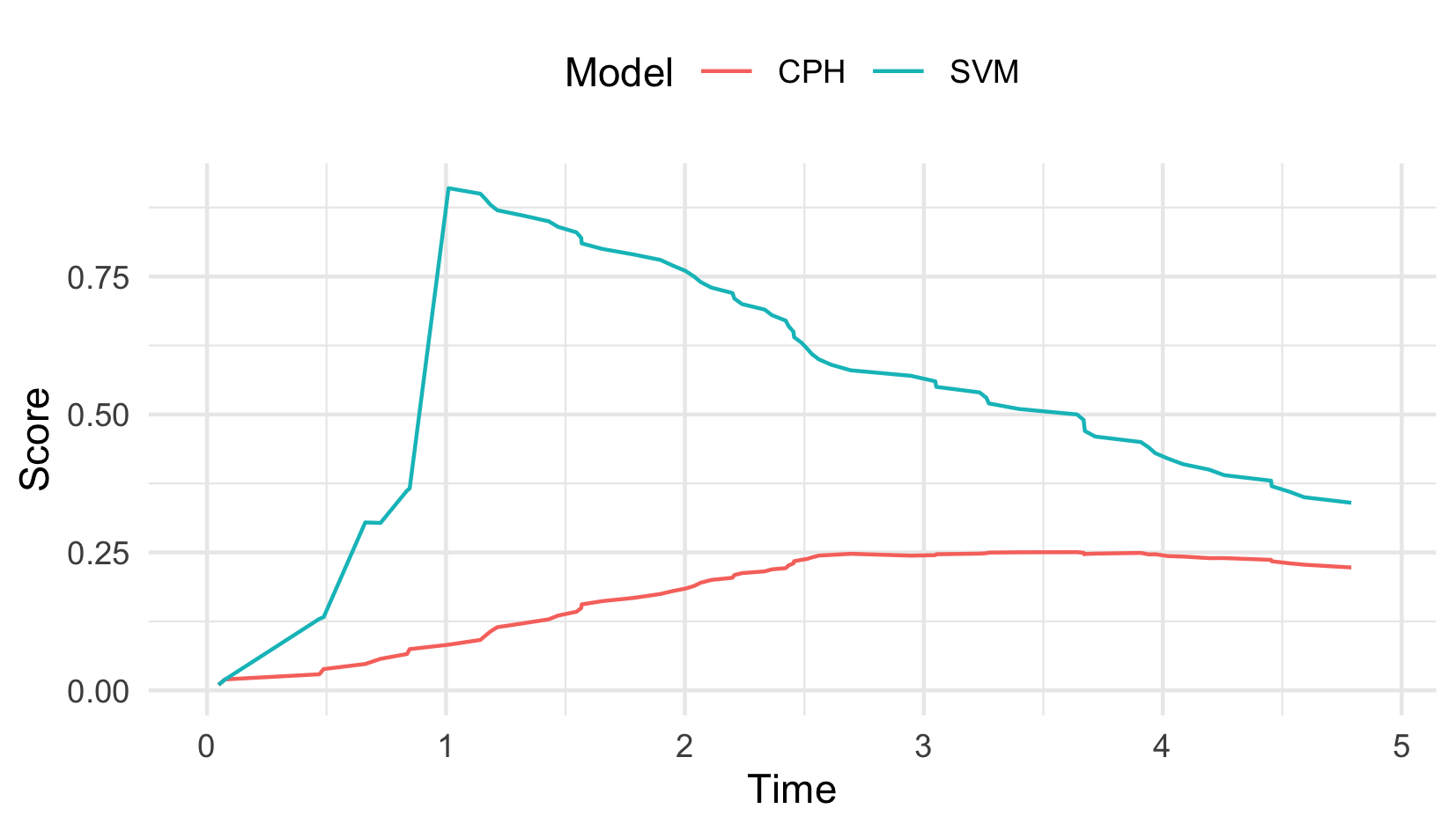
As well as evaluating probabilistic outcomes with integrated scoring rules, non-integrated scoring rules can be utilised for evaluating distributions at a single point. For example, instead of evaluating a probabilistic prediction with the IGS over \(\mathbb{R}_{\geq 0}\), instead one could compute the IGS at a single time-point, \(\tau \in \mathbb{R}_{\geq 0}\), only. Plotting these for varying values of \(\tau\) results in ‘prediction error curves’ (PECs), which provide a simple visualisation for how predictions vary over the outcome. PECs are especially useful for survival predictions as they can visualise the prediction ‘over time’. PECs are mostly used as a graphical guide when comparing few models, rather than as a formal tool for model comparison. An example for PECs is provided in Figure 10.2 for the IGS where the the Cox PH consistently outperforms the SVM.
10.4 Baselines and ERV
A common criticism of scoring rules is a lack of interpretability, for example, an IGS of 0.5 or 0.0005 has no meaning by itself, so below we present two methods to help overcome this problem.
The first method, is to make use of baselines for model comparison, which are models or values that can be utilised to provide a reference for a loss, they provide a universal method to judge all models of the same class by (Gressmann et al. 2018). In classification, it is possible to derive analytical baseline values, for example a Brier score is considered ‘good’ if it is below 0.25 or a log loss if it is below 0.693 (Figure 10.1), this is because these are the values obtained if you always predicted probabilties as \(0.5\), which is a reasonable basline guess in a binary classificaiton problem. In survival analysis, simple analytical expressions are not possible as losses are dependent on the unknown distributions of both the survival and censoring time. Therefore all experiments in survival analysis must include a baseline model that can produce a reference value in order to derive meaningful results. A suitable baseline model is the Kaplan-Meier estimator (Graf and Schumacher 1995; Lawless and Yuan 2010; Royston and Altman 2013), which is the simplest model that can consistently estimate the true survival function.
As well as directly comparing losses from a ‘sophisticated’ model to a baseline, one can also compute the percentage increase in performance between the sophisicated and baseline models, which produces a measure of explained residual variation (ERV) (Edward L. Korn and Simon 1990; Edward L. Korn and Simon 1991). For any survival loss \(L\), the ERV is,
\[ R_L(S, B) = 1 - \frac{L|S}{L|B} \]
where \(L|S\) and \(L|B\) is the loss computed with respect to predictions from the sophisticated and baseline models respectively.
The ERV interpretation makes reporting of scoring rules easier within and between experiments. For example, say in experiment A we have \(L|S = 0.004\) and \(L|B = 0.006\), and in experiment B we have \(L|S = 4\) and \(L|B = 6\). The sophisticated model may appear worse at first glance in experiment A (as the losses are very close) but when considering the ERV we see that the performance increase is identical (both \(R_L = 33\%\)), thus providing a clearer way to compare models.